• 109
C h a p t e r
5
Diffusion
P
hotograph of a steel gear that has been “case hardened.” The outer surface layer was selectively hardened by a high-temperature heat treatment during which carbon from the sur-rounding atmosphere diffused into the surface. The “case” appears as the dark outer rim of that segment of the gear that has been sectioned. Actual size. (Photograph courtesy of Surface Division Midland-Ross.)Materials of all types are often heat treated to im-prove their properties. The phenomena that occur during a heat treatment almost always involve atomic diffusion. Often an enhancement of diffusion rate is desired; on occasion measures are taken to reduce it. Heat-treating temperatures and times, and/or cooling
rates are often predictable using the mathematics of diffusion and appropriate diffusion constants. The steel gear shown on this page has been case hardened (Section 8.10); that is, its hardness and resistance to failure by fatigue have been enhanced by diffusing excess carbon or nitrogen into the outer surface layer.
5.1 INTRODUCTION
Many reactions and processes that are important in the treatment of materials rely on the transfer of mass either within a specific solid (ordinarily on a microscopic level) or from a liquid, a gas, or another solid phase. This is necessarily accomplished by diffusion,the phenomenon of material transport by atomic motion. This chapter dis-cusses the atomic mechanisms by which diffusion occurs, the mathematics of diffu-sion, and the influence of temperature and diffusing species on the rate of diffusion. The phenomenon of diffusion may be demonstrated with the use of a diffusion
couple, which is formed by joining bars of two different metals together so that
there is intimate contact between the two faces; this is illustrated for copper and nickel in Figure 5.1, which includes schematic representations of atom positions and composition across the interface. This couple is heated for an extended period at an elevated temperature (but below the melting temperature of both metals), and L e a r n i n g O b j e c t i v e s
After studying this chapter you should be able to do the following: 1. Name and describe the two atomic mechanisms
of diffusion.
2. Distinguish between steady-state and nonsteady-state diffusion.
3. (a) Write Fick’s first and second laws in equa-tion form, and define all parameters. (b) Note the kind of diffusion for which each
of these equations is normally applied.
4. Write the solution to Fick’s second law for diffusion into a semi-infinite solid when the concentration of diffusing species at the surface is held constant. Define all parameters in this equation.
5. Calculate the diffusion coefficient for some material at a specified temperature, given the appropriate diffusion constants.
Cu Ni
Cu Ni
100
0
Concentration of Ni, Cu
Position
(c) (b) (a) diffusion
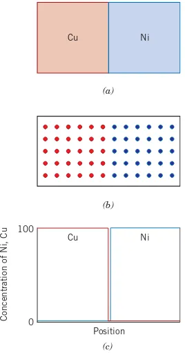
Figure 5.1 (a) A copper–nickel diffusion couple before a high-temperature heat treatment. (b) Schematic representations of Cu (red
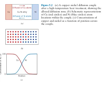
cooled to room temperature. Chemical analysis will reveal a condition similar to that represented in Figure 5.2—namely, pure copper and nickel at the two extrem-ities of the couple, separated by an alloyed region. Concentrations of both metals vary with position as shown in Figure 5.2c. This result indicates that copper atoms have migrated or diffused into the nickel, and that nickel has diffused into copper. This process, whereby atoms of one metal diffuse into another, is termed interdif-fusion,orimpurity diffusion.
Interdiffusion may be discerned from a macroscopic perspective by changes in concentration which occur over time, as in the example for the Cu–Ni diffusion cou-ple. There is a net drift or transport of atoms from high- to low-concentration re-gions. Diffusion also occurs for pure metals, but all atoms exchanging positions are of the same type; this is termed self-diffusion.Of course, self-diffusion is not nor-mally subject to observation by noting compositional changes.
5.2 DIFFUSION MECHANISMS
From an atomic perspective, diffusion is just the stepwise migration of atoms from lattice site to lattice site. In fact, the atoms in solid materials are in constant mo-tion, rapidly changing positions. For an atom to make such a move, two conditions must be met: (1) there must be an empty adjacent site, and (2) the atom must have sufficient energy to break bonds with its neighbor atoms and then cause some lat-tice distortion during the displacement. This energy is vibrational in nature (Sec-tion 4.8). At a specific temperature some small frac(Sec-tion of the total number of atoms is capable of diffusive motion, by virtue of the magnitudes of their vibrational energies. This fraction increases with rising temperature.
Several different models for this atomic motion have been proposed; of these possibilities, two dominate for metallic diffusion.
5.2 Diffusion Mechanisms • 111 Figure 5.2 (a) A copper–nickel diffusion couple after a high-temperature heat treatment, showing the alloyed diffusion zone. (b) Schematic representations of Cu (red circles) and Ni (blue circles) atom locations within the couple. (c) Concentrations of copper and nickel as a function of position across the couple.
Concentration of Ni, Cu
Position Ni Cu
0 100
(c) (b) (a) Diffusion of Ni atoms Diffusion of Cu atoms
Cu-Ni alloy Ni Cu
interdiffusion
impurity diffusion
Vacancy Diffusion
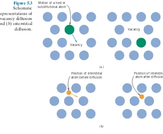
One mechanism involves the interchange of an atom from a normal lattice position to an adjacent vacant lattice site or vacancy, as represented schematically in Fig-ure 5.3a. This mechanism is aptly termed vacancy diffusion.Of course, this process necessitates the presence of vacancies, and the extent to which vacancy diffusion can occur is a function of the number of these defects that are present; significant concentrations of vacancies may exist in metals at elevated temperatures (Section 4.2). Since diffusing atoms and vacancies exchange positions, the diffusion of atoms in one direction corresponds to the motion of vacancies in the opposite direction. Both self-diffusion and interdiffusion occur by this mechanism; for the latter, the impu-rity atoms must substitute for host atoms.
Interstitial Diffusion
The second type of diffusion involves atoms that migrate from an interstitial posi-tion to a neighboring one that is empty. This mechanism is found for interdiffusion of impurities such as hydrogen, carbon, nitrogen, and oxygen, which have atoms that are small enough to fit into the interstitial positions. Host or substitutional im-purity atoms rarely form interstitials and do not normally diffuse via this mecha-nism. This phenomenon is appropriately termed interstitial diffusion(Figure 5.3b). In most metal alloys, interstitial diffusion occurs much more rapidly than diffu-sion by the vacancy mode, since the interstitial atoms are smaller and thus more mo-bile. Furthermore, there are more empty interstitial positions than vacancies; hence, the probability of interstitial atomic movement is greater than for vacancy diffusion.
5.3 STEADY-STATE DIFFUSION
Diffusion is a time-dependent process—that is, in a macroscopic sense, the quan-tity of an element that is transported within another is a function of time. Often it Motion of a host or
substitutional atom
Vacancy
Vacancy
Position of interstitial atom after diffusion Position of interstitial
atom before diffusion (a )
(b) Figure 5.3
Schematic representations of (a) vacancy diffusion and (b) interstitial diffusion.
vacancy diffusion
5.3 Steady-State Diffusion • 113 is necessary to know how fast diffusion occurs, or the rate of mass transfer. This rate is frequently expressed as a diffusion flux(J), defined as the mass (or, equiva-lently, the number of atoms) M diffusing through and perpendicular to a unit cross-sectional area of solid per unit of time. In mathematical form, this may be represented as
(5.1a)
whereAdenotes the area across which diffusion is occurring and tis the elapsed diffusion time. In differential form, this expression becomes
(5.1b)
The units for Jare kilograms or atoms per meter squared per second (kg/m2-s or atoms/m2-s).
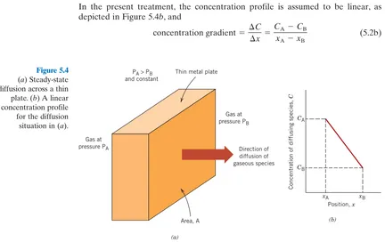
If the diffusion flux does not change with time, a steady-state condition exists. One common example of steady-state diffusionis the diffusion of atoms of a gas through a plate of metal for which the concentrations (or pressures) of the diffus-ing species on both surfaces of the plate are held constant. This is represented schematically in Figure 5.4a.
When concentration Cis plotted versus position (or distance) within the solid
x, the resulting curve is termed the concentration profile;the slope at a particular point on this curve is the concentration gradient:
(5.2a)
In the present treatment, the concentration profile is assumed to be linear, as depicted in Figure 5.4b, and
(5.2b) concentration gradient⫽¢C
¢x ⫽
CA⫺CB
xA⫺xB
concentration gradient⫽dC
dx
J⫽ 1
A dM
dt
J⫽ M
At Definition of
diffusion flux
steady-state diffusion
concentration profile
concentration gradient
xA xB
Position,x
Concentration of diffusing species,
C
(b)
(a)
CA
CB Thin metal plate
Area, A
Direction of diffusion of gaseous species Gas at
pressure PB
Gas at pressure PA
PA> PB
and constant Figure 5.4
For diffusion problems, it is sometimes convenient to express concentration in terms of mass of diffusing species per unit volume of solid (kg/m3or g/cm3).1
The mathematics of steady-state diffusion in a single (x) direction is relatively simple, in that the flux is proportional to the concentration gradient through the expression
(5.3)
The constant of proportionality Dis called the diffusion coefficient,which is ex-pressed in square meters per second. The negative sign in this expression indicates that the direction of diffusion is down the concentration gradient, from a high to a low concentration. Equation 5.3 is sometimes called Fick’s first law.
Sometimes the term driving forceis used in the context of what compels a re-action to occur. For diffusion rere-actions, several such forces are possible; but when diffusion is according to Equation 5.3, the concentration gradient is the driving force. One practical example of steady-state diffusion is found in the purification of hydrogen gas. One side of a thin sheet of palladium metal is exposed to the impure gas composed of hydrogen and other gaseous species such as nitrogen, oxygen, and water vapor. The hydrogen selectively diffuses through the sheet to the opposite side, which is maintained at a constant and lower hydrogen pressure.
EXAMPLE PROBLEM 5.1
Diffusion Flux Computation
A plate of iron is exposed to a carburizing (carbon-rich) atmosphere on one side and a decarburizing (carbon-deficient) atmosphere on the other side at ( ). If a condition of steady state is achieved, calculate the diffu-sion flux of carbon through the plate if the concentrations of carbon at positions of 5 and 10 mm ( and ) beneath the carburizing surface are 1.2 and 0.8 kg/m3, respectively. Assume a diffusion coefficient of
at this temperature.
Solution
Fick’s first law, Equation 5.3, is utilized to determine the diffusion flux. Sub-stitution of the values above into this expression yields
5.4 NONSTEADY-STATE DIFFUSION
Most practical diffusion situations are nonsteady-state ones. That is, the diffusion flux and the concentration gradient at some particular point in a solid vary with time, with a net accumulation or depletion of the diffusing species resulting. This is illustrated in Figure 5.5, which shows concentration profiles at three different
⫽2.4⫻10⫺9 kg/m2-s
J⫽ ⫺DCA
⫺CB
xA⫺xB
⫽ ⫺13⫻10⫺11 m2/s2 11.2
⫺0.82 kg/m3 15⫻10⫺3⫺10⫺22 m
3⫻10⫺11 m2/s 10⫺2 m
5⫻10⫺3 1300⬚F
700⬚C
J⫽ ⫺DdC
dx Fick’s first law—
diffusion flux for steady-state diffusion (in one direction)
diffusion coefficient
driving force Fick’s first law
1Conversion of concentration from weight percent to mass per unit volume (in kg/m3) is
diffusion times. Under conditions of nonsteady state, use of Equation 5.3 is no longer convenient; instead, the partial differential equation
(5.4a)
known as Fick’s second law,is used. If the diffusion coefficient is independent of composition (which should be verified for each particular diffusion situation), Equation 5.4a simplifies to
(5.4b)
Solutions to this expression (concentration in terms of both position and time) are possible when physically meaningful boundary conditions are specified. Comprehen-sive collections of these are given by Crank, and Carslaw and Jaeger (see References). One practically important solution is for a semi-infinite solid2in which the sur-face concentration is held constant. Frequently, the source of the diffusing species is a gas phase, the partial pressure of which is maintained at a constant value. Fur-thermore, the following assumptions are made:
1. Before diffusion, any of the diffusing solute atoms in the solid are uniformly distributed with concentration of
2. The value of xat the surface is zero and increases with distance into the solid. 3. The time is taken to be zero the instant before the diffusion process begins.
These boundary conditions are simply stated as
Application of these boundary conditions to Equation 5.4b yields the solution
(5.5)
Cx⫺C0
Cs⫺C0⫽1⫺erfa
x
21Dtb
C⫽C0 at x⫽q
For t 7 0,C⫽C
s1the constant surface concentration2 at x⫽0
For t⫽0,C⫽C0 at 0ⱕxⱕq
C0.
0C
0t ⫽D 02C
0x2
0C
0t ⫽ 0
0xaD 0C
0xb
5.4 Nonsteady-State Diffusion • 115
Fick’s second law
Fick’s second law— diffusion equation for nonsteady-state diffusion (in one direction)
2A bar of solid is considered to be semi-infinite if none of the diffusing atoms reaches the
bar end during the time over which diffusion takes place. A bar of length lis considered to be semi-infinite when l7 101Dt.
Figure 5.5 Concentration profiles for nonsteady-state diffusion taken at three different times,t1,t2,and t3.
Distance
Concentration of diffusing species
t3>t2>t1
t2 t1
t3
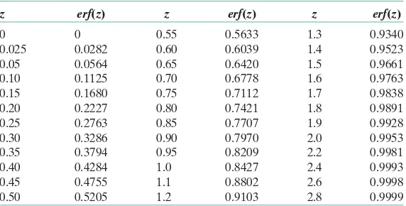
where represents the concentration at depth x after time t. The expression erf( ) is the Gaussian error function,3values of which are given in mathe-matical tables for various values; a partial listing is given in Table 5.1. The concentration parameters that appear in Equation 5.5 are noted in Figure 5.6, a concentration profile taken at a specific time. Equation 5.5 thus demonstrates the relationship between concentration, position, and time—namely, that being a function of the dimensionless parameter may be determined at any time and position if the parameters and Dare known.
Suppose that it is desired to achieve some specific concentration of solute, in an alloy; the left-hand side of Equation 5.5 now becomes
This being the case, the right-hand side of this same expression is also a constant, and subsequently
(5.6a)
x
21Dt
⫽constant
C1⫺C0
Cs⫺C0
⫽constant
C1,
Cs,
C0,
x
Ⲑ
1Dt,Cx,
x
Ⲑ
21Dtx
Ⲑ
21DtCx
Table 5.1 Tabulation of Error Function Values
z erf(z) z erf(z) z erf(z)
0 0 0.55 0.5633 1.3 0.9340
0.025 0.0282 0.60 0.6039 1.4 0.9523
0.05 0.0564 0.65 0.6420 1.5 0.9661
0.10 0.1125 0.70 0.6778 1.6 0.9763
0.15 0.1680 0.75 0.7112 1.7 0.9838
0.20 0.2227 0.80 0.7421 1.8 0.9891
0.25 0.2763 0.85 0.7707 1.9 0.9928
0.30 0.3286 0.90 0.7970 2.0 0.9953
0.35 0.3794 0.95 0.8209 2.2 0.9981
0.40 0.4284 1.0 0.8427 2.4 0.9993
0.45 0.4755 1.1 0.8802 2.6 0.9998
0.50 0.5205 1.2 0.9103 2.8 0.9999
3This Gaussian error function is defined by
where x
Ⲑ
21Dthas been replaced by the variable z. erf1z2⫽ 21p
冮
z
0e
⫺y2
dy
Distance from interface, x
Concentration,
C
Cx – C0
C0 Cx
Cs
Cs – C0
or
(5.6b)
Some diffusion computations are thus facilitated on the basis of this relation-ship, as demonstrated in Example Problem 5.3.
EXAMPLE PROBLEM 5.2
Nonsteady-State Diffusion Time Computation I
For some applications, it is necessary to harden the surface of a steel (or iron-carbon alloy) above that of its interior. One way this may be accomplished is by increasing the surface concentration of carbon in a process termed car-burizing;the steel piece is exposed, at an elevated temperature, to an atmo-sphere rich in a hydrocarbon gas, such as methane
Consider one such alloy that initially has a uniform carbon concentration of 0.25 wt% and is to be treated at 950 C (1750 F). If the concentration of carbon at the surface is suddenly brought to and maintained at 1.20 wt%, how long will it take to achieve a carbon content of 0.80 wt% at a position 0.5 mm below the surface? The diffusion coefficient for carbon in iron at this tem-perature is m2/s; assume that the steel piece is semi-infinite.
Solution
Since this is a nonsteady-state diffusion problem in which the surface com-position is held constant, Equation 5.5 is used. Values for all the parameters in this expression except time tare specified in the problem as follows:
Thus,
We must now determine from Table 5.1 the value of z for which the error function is 0.4210. An interpolation is necessary, as
z erf(z)
0.35 0.3794
z 0.4210
0.40 0.4284
z⫺0.35
0.40⫺0.35⫽
0.4210⫺0.3794 0.4284⫺0.3794 0.4210⫽erfa62.5 s
1Ⲑ2
1t b
Cx⫺C0
Cs⫺C0
⫽0.80⫺0.25
1.20⫺0.25⫽1⫺erf c
15⫻10⫺4 m2 2211.6⫻10⫺11 m2/s21t2d
D⫽1.6⫻10⫺11 m2/s
x⫽0.50 mm⫽5⫻10⫺4 m
Cx⫽0.80 wt% C
Cs⫽1.20 wt% C
C0⫽0.25 wt% C 1.6⫻10⫺11
⬚ ⬚
1CH42.
x2
Dt⫽constant
5.4 Nonsteady-State Diffusion • 117
or
Therefore,
and solving for t,
EXAMPLE PROBLEM 5.3
Nonsteady-State Diffusion Time Computation II
The diffusion coefficients for copper in aluminum at 500 and 600 C are 4.8 and 5.3 m2/s, respectively. Determine the approximate time at 500 C that will produce the same diffusion result (in terms of concentra-tion of Cu at some specific point in Al) as a 10-h heat treatment at 600°C.
Solution
This is a diffusion problem in which Equation 5.6b may be employed. The composition in both diffusion situations will be equal at the same position (i.e.,
xis also a constant), thus
(5.7)
at both temperatures. That is,
or
5.5 FACTORS THAT INFLUENCE DIFFUSION
Diffusing Species
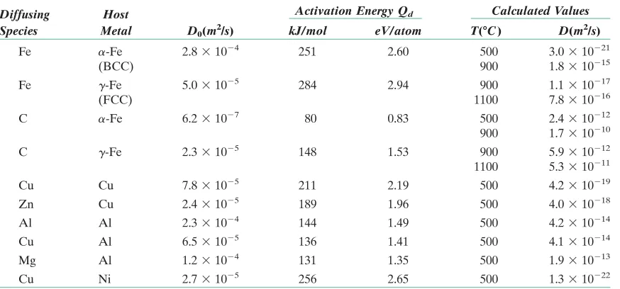
The magnitude of the diffusion coefficient Dis indicative of the rate at which atoms diffuse. Coefficients, both self- and interdiffusion, for several metallic systems are listed in Table 5.2. The diffusing species as well as the host material influence the diffu-sion coefficient. For example, there is a significant difference in magnitude between self-diffusion and carbon interdiffusion in iron at 500 C, the Dvalue being greater for the carbon interdiffusion ( vs. ). This comparison also provides a contrast between rates of diffusion via vacancy and interstitial modes as discussed above. Self-diffusion occurs by a vacancy mechanism, whereas carbon diffusion in iron is interstitial.
Temperature
Temperature has a most profound influence on the coefficients and diffusion rates. For example, for the self-diffusion of Fe in -Fe, the diffusion coefficient increases approximately six orders of magnitude (from 3.0 to 1.8 in rising temperature from 500 to 900 C (Table 5.2). The temperature dependence of⬚
m2/s2
⫻10⫺15
⫻10⫺21 a
m2/s 2.4⫻10⫺12 3.0⫻10⫺21
⬚ a
t500⫽
D600t600
D500
⫽ 15.3
⫻10⫺13 m2/s2110 h2
4.8⫻10⫺14 m2/s ⫽110.4 h
D500t500⫽D600t600
Dt⫽constant ⬚
⫻10⫺13
⫻10⫺14
⬚
t⫽a62.5 s
1Ⲑ2
0.392 b 2
⫽25,400 s⫽7.1 h 62.5 s1Ⲑ2
1t
⫽0.392
the diffusion coefficients is
(5.8)
where
a temperature-independent preexponential
theactivation energyfor diffusion (J/mol or eV/atom)
R⫽ the gas constant, 8.31 J/mol-K or 8.62 eV/atom-K
T⫽ absolute temperature (K)
The activation energy may be thought of as that energy required to produce the diffusive motion of one mole of atoms. A large activation energy results in a relatively small diffusion coefficient. Table 5.2 also contains a listing of and values for several diffusion systems.
Taking natural logarithms of Equation 5.8 yields
(5.9a)
or in terms of logarithms to the base 10
(5.9b)
Since , and Rare all constants, Equation 5.9b takes on the form of an equa-tion of a straight line:
whereyandxare analogous, respectively, to the variables log Dand Thus, if logDis plotted versus the reciprocal of the absolute temperature, a straight line
1
Ⲑ
T.y⫽b⫹mx
Qd
D0,
logD⫽logD0⫺ Qd 2.3Ra
1
Tb
lnD⫽lnD0⫺Qd
R a
1
Tb
Qd
D0
⫻10⫺5
Qd⫽
1m2/s2
D0⫽
D⫽D0expa⫺Qd
RTb
5.5 Factors That Influence Diffusion • 119 Table 5.2 A Tabulation of Diffusion Data
Diffusing Host Activation Energy Qd Calculated Values
Species Metal D0(m2/s) kJ/mol eV/atom T(ⴗC) D(m2/s)
Fe ␣-Fe 2.8⫻ 10⫺4 251 2.60 500 3.0⫻ 10⫺21
(BCC) 900 1.8⫻ 10⫺15
Fe ␥-Fe 5.0⫻ 10⫺5 284 2.94 900 1.1⫻ 10⫺17
(FCC) 1100 7.8⫻ 10⫺16
C ␣-Fe 6.2⫻ 10⫺7 80 0.83 500 2.4⫻ 10⫺12
900 1.7⫻ 10⫺10
C ␥-Fe 2.3⫻ 10⫺5 148 1.53 900 5.9⫻ 10⫺12
1100 5.3⫻ 10⫺11
Cu Cu 7.8⫻ 10⫺5 211 2.19 500 4.2⫻ 10⫺19
Zn Cu 2.4⫻ 10⫺5 189 1.96 500 4.0⫻ 10⫺18
Al Al 2.3⫻ 10⫺4 144 1.49 500 4.2⫻ 10⫺14
Cu Al 6.5⫻ 10⫺5 136 1.41 500 4.1⫻ 10⫺14
Mg Al 1.2⫻ 10⫺4 131 1.35 500 1.9⫻ 10⫺13
Cu Ni 2.7⫻ 10⫺5 256 2.65 500 1.3⫻ 10⫺22
Source:E. A. Brandes and G. B. Brook (Editors),Smithells Metals Reference Book,7th edition, Butterworth-Heinemann, Oxford, 1992.
Dependence of the diffusion coefficient on temperature
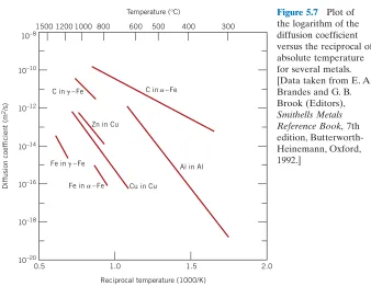
should result, having slope and intercept of and log respectively. This is, in fact, the manner in which the values of and are determined experi-mentally. From such a plot for several alloy systems (Figure 5.7), it may be noted that linear relationships exist for all cases shown.
Concept Check 5.1
Rank the magnitudes of the diffusion coefficients from greatest to least for the fol-lowing systems:
N in Fe at 700°C Cr in Fe at 700°C N in Fe at 900°C Cr in Fe at 900°C
Now justify this ranking. (Note:Both Fe and Cr have the BCC crystal structure, and the atomic radii for Fe, Cr, and N are 0.124, 0.125, and 0.065 nm, respectively. You may also want to refer to Section 4.3.)
[The answer may be found at www.wiley.com/college/callister(Student Companion Site).]
Concept Check 5.2
Consider the self-diffusion of two hypothetical metals A and B. On a schematic graph of ln D versus , plot (and label) lines for both metals given that
and also that
[The answer may be found at www.wiley.com/college/callister(Student Companion Site).]
Qd1A2 7 Q
d1B2.
D01A2 7 D01B2
1
Ⲑ
TD0
Qd
D0,
⫺Qd
Ⲑ
2.3R1500 1200 1000 800 600 500 400 300
Diffusion coefficient (m
2/s) 10–8
10–10
10–12
10–14
10–16
10–18
10–20
Temperature (°C)
Reciprocal temperature (1000/K)
0.5 1.0 1.5 2.0
Al in Al Zn in Cu
Cu in Cu C in –Fe␥
Fe in –Fe␥
C in –Fe␣
Fe in –Fe␣
Figure 5.7 Plot of the logarithm of the diffusion coefficient versus the reciprocal of absolute temperature for several metals. [Data taken from E. A. Brandes and G. B. Brook (Editors),
EXAMPLE PROBLEM 5.4
Diffusion Coefficient Determination
Using the data in Table 5.2, compute the diffusion coefficient for magnesium in aluminum at 550 C.
Solution
This diffusion coefficient may be determined by applying Equation 5.8; the values of and from Table 5.2 are 1.2 m2/s and 131 kJ/mol, respectively. Thus,
EXAMPLE PROBLEM 5.5
Diffusion Coefficient Activation Energy and Preexponential Calculations
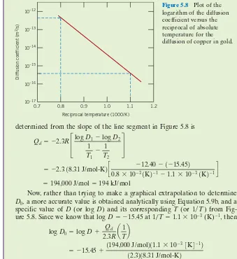
In Figure 5.8 is shown a plot of the logarithm (to the base 10) of the diffusion coefficient versus reciprocal of absolute temperature, for the diffusion of cop-per in gold. Determine values for the activation energy and the preexponential.
Solution
From Equation 5.9b the slope of the line segment in Figure 5.8 is equal to , and the intercept at gives the value of log Thus, the activation energy may be determined as
where and are the diffusion coefficient values at and
re-spectively. Let us arbitrarily take and
We may now read the corresponding log and log values from the line segment in Figure 5.8.
[Before this is done, however, a parenthetic note of caution is offered. The vertical axis in Figure 5.8 is scaled logarithmically (to the base 10); however, the actual diffusion coefficient values are noted on this axis. For example, for m2/s, the logarithm of Dis not Furthermore, this log-arithmic scaling affects the readings between decade values; for example, at a location midway between and the value is not but, rather,
].
Thus, from Figure 5.8, at log while
for 1
Ⲑ
T2⫽1.1⫻10 log D2⫽ ⫺15.45, and the activation energy, as5.5 Factors That Influence Diffusion • 121
D0andQdfrom
DESIGN EXAMPLE 5.1
Diffusion Temperature–Time Heat Treatment Specification
The wear resistance of a steel gear is to be improved by hardening its surface. This is to be accomplished by increasing the carbon content within an outer surface layer as a result of carbon diffusion into the steel; the carbon is to be supplied from an external carbon-rich gaseous atmosphere at an elevated and constant temperature. The initial carbon content of the steel is 0.20 wt%, whereas the surface concentration is to be maintained at 1.00 wt%. For this treatment to be effective, a carbon content of 0.60 wt% must be established at a position 0.75 mm below the surface. Specify an appropriate heat treatment in terms of temperature and time for temperatures between 900 C and 1050 C. Use data in Table 5.2 for the diffusion of carbon in -iron.g
⬚ ⬚
determined from the slope of the line segment in Figure 5.8 is
Now, rather than trying to make a graphical extrapolation to determine a more accurate value is obtained analytically using Equation 5.9b, and a specific value of D(or log D) and its corresponding T (or 1兾T) from
Fig-ure 5.8. Since we know that log at (K) then
Thus,D m2/s⫽5.2⫻10⫺5m2/s. 0⫽10
⫺4.28
⫽ ⫺4.28
⫽ ⫺15.45⫹ 1194,000 J/mol211.1
⫻10⫺33K4⫺12 12.3218.31 J/mol-K2 log D0⫽logD⫹
Qd
2.3Ra
1
Tb
⫺1, 1
Ⲑ
T⫽1.1⫻10⫺3D⫽ ⫺15.45
D0,
⫽194,000 J/mol⫽194 kJ/mol ⫽ ⫺2.318.31 J/mol-K2 c
⫺12.40⫺1⫺15.452
0.8⫻10⫺31K2⫺1⫺1.1⫻10⫺31K2⫺1d
Qd⫽ ⫺2.3R£
logD1⫺logD2 1
T1⫺
1
T2
§
0.7 0.8 0.9 1.0 1.1 1.2
Diffusion coefficient (m
2/s) 10–12
10–13
10–15 10–14
10–16
10–17
Reciprocal temperature (1000/K)
5.5 Factors That Influence Diffusion • 123
Solution
Since this is a nonsteady-state diffusion situation, let us first of all employ Equa-tion 5.5, utilizing the following values for the concentraEqua-tion parameters:
Therefore
and thus
Using an interpolation technique as demonstrated in Example Problem 5.2 and the data presented in Table 5.1,
(5.10)
The problem stipulates that mm m. Therefore
This leads to
Furthermore, the diffusion coefficient depends on temperature according to Equation 5.8; and, from Table 5.2 for the diffusion of carbon in -iron,
m2/s and J/mol. Hence
and solving for the time t
Thus, the required diffusion time may be computed for some specified temper-ature (in K). Below are tabulated tvalues for four different temperatures that lie within the range stipulated in the problem.
Temperature Time
(ⴗC) s h
900 106,400 29.6
950 57,200 15.9
1000 32,300 9.0
1050 19,000 5.3
t1in s2⫽ 0.0271 expa⫺17,810
T b
12.3⫻10⫺5 m2/s2 exp c⫺ 148,000 J/mol
18.31 J/mol-K21T2 d 1t2⫽6.24⫻10
⫺7 m2
Dt⫽D0 exp a⫺Qd
RTb 1t2⫽6.24⫻10
⫺7 m2
Qd⫽148,000
D0⫽2.3⫻10
⫺5
g
Dt⫽6.24⫻10⫺7 m2
7.5⫻10⫺4 m 21Dt
⫽0.4747 ⫽7.5⫻10⫺4
x⫽0.75
x
21Dt
⫽0.4747 0.5⫽erfa x
21Dtb
Cx⫺C0
Cs⫺C0⫽
0.60⫺0.20
1.00⫺0.20⫽1⫺erfa
x
21Dtb Cx⫽0.60 wt% C
Aluminum for Integrated Circuit Interconnects
MATERIAL OF IMPORTANCE
Interconnects
Figure 5.9 Scanning electron micrograph of an inte-grated circuit chip, on which is noted aluminum inter-connect regions. Approximately 2000⫻. (Photograph
courtesy of National Semiconductor Corporation.)
10–12 1200 1000 900 800 700 600 500 400
Temperature (°C)
Cu in Si
Figure 5.10 Logarithm of D-versus- (K) curves (lines) for the diffusion of copper, gold, silver, and aluminum in silicon. Also noted are Dvalues at 500 C.⬚
1
Ⲑ
TT
he heart of all computers and other electronic devices is the integrated circuit(orIC).4Each integrated circuit chip is a thin square wafer hav-ing dimensions on the order of 6 mm by 6 mm by 0.4 mm; furthermore, literally millions of inter-connected electronic components and circuits are embedded in one of the chip faces. The base ma-terial for ICs is silicon, to which has been added very specific and extremely minute and controlled concentrations of impurities that are confined to very small and localized regions. For some ICs, the impurities are added using high-temperature dif-fusion heat treatments.One important step in the IC fabrication process is the deposition of very thin and narrow conducting circuit paths to facilitate the passage of current from one device to another; these paths are called “interconnects,” and several are shown in Figure 5.9, a scanning electron micrograph of an IC chip. Of course the material to be used for interconnects must have a high electrical conduc-tivity—a metal, since, of all materials, metals have the highest conductivities. Table 5.3 cites values for silver, copper, gold, and aluminum, the most conductive metals.
On the basis of these conductivities, and dis-counting material cost, Ag is the metal of choice, followed by Cu, Au, and Al.
Once these interconnects have been de-posited, it is still necessary to subject the IC chip to other heat treatments, which may run as high as 500 C. If, during these treatments, there is signifi-cant diffusion of the interconnect metal into the silicon, the electrical functionality of the IC will be destroyed. Thus, since the extent of diffusion is de-pendent on the magnitude of the diffusion coeffi-cient, it is necessary to select an interconnect metal that has a small value of Din silicon. Figure 5.10
⬚
Table 5.3 Room-Temperature Electrical Con-ductivity Values for Silver, Copper, Gold, and Aluminum (the Four Most Conductive Metals)
Summary • 125
plots the logarithm of Dversus for the diffu-sion, into silicon, of copper, gold, silver, and alu-minum. Also, a dashed vertical line has been constructed at 500 C, from which values of D, for the four metals are noted at this temperature. Here it may be seen that the diffusion coefficient for alu-minum in silicon ( m2/s) is at least four orders of magnitude (i.e., a factor of 104) lower than the values for the other three metals.
Aluminum is indeed used for interconnects in some integrated circuits; even though its electrical conductivity is slightly lower than the values for
2.5⫻10⫺21
⬚
1
Ⲑ
T silver, copper, and gold, its extremely low diffusion coefficient makes it the material of choice for this application. An aluminum-copper-silicon alloy (Al-4 wt% Cu-1.5 wt% Si) is sometimes also used for interconnects; it not only bonds easily to the surface of the chip, but is also more corrosion re-sistant than pure aluminum.More recently, copper interconnects have also been used. However, it is first necessary to deposit a very thin layer of tantalum or tantalum nitride beneath the copper, which acts as a barrier to deter diffusion of Cu into the silicon.
5.6 OTHER DIFFUSION PATHS
Atomic migration may also occur along dislocations, grain boundaries, and exter-nal surfaces. These are sometimes called “short-circuit”diffusion paths inasmuch as rates are much faster than for bulk diffusion. However, in most situations short-circuit contributions to the overall diffusion flux are insignificant because the cross-sectional areas of these paths are extremely small.
S U M M A RY
Diffusion Mechanisms
Solid-state diffusion is a means of mass transport within solid materials by stepwise atomic motion. The term “self-diffusion” refers to the migration of host atoms; for impurity atoms, the term “interdiffusion” is used. Two mechanisms are possible: va-cancy and interstitial. For a given host metal, interstitial atomic species generally diffuse more rapidly.
Steady-State Diffusion Nonsteady-State Diffusion
For steady-state diffusion, the concentration profile of the diffusing species is time independent, and the flux or rate is proportional to the negative of the concen-tration gradient according to Fick’s first law. The mathematics for nonsteady state are described by Fick’s second law, a partial differential equation. The solution for a constant surface composition boundary condition involves the Gaussian error function.
Factors That Influence Diffusion
Activation energy
Fick’s first and second laws Interdiffusion (impurity diffusion)
Gale, W. F. and T. C. Totemeier, (Editors),Smithells
Metals Reference Book,8th
edition,Butterworth-Heinemann Ltd, Woburn, UK, 2004.
Carslaw, H. S. and J. C. Jaeger,Conduction of Heat
in Solids,2nd edition, Oxford University Press,
Oxford, 1986.
Crank, J.,The Mathematics of Diffusion,2nd edi-tion, Oxford University Press, Oxford, 1980.
Glicksman, M., Diffusion in Solids, Wiley-Interscience, New York, 2000.
Shewmon, P. G.,Diffusion in Solids,2nd edition, The Minerals, Metals and Materials Society, Warrendale, PA, 1989.
Q U E S T I O N S A N D P R O B L E M S
Introduction
5.1 Briefly explain the difference between self-diffusion and interself-diffusion.
5.2 Self-diffusion involves the motion of atoms that are all of the same type; therefore it is not subject to observation by compositional changes, as with interdiffusion. Suggest one way in which self-diffusion may be monitored.
Diffusion Mechanisms
5.3 (a) Compare interstitial and vacancy atomic mechanisms for diffusion.
(b) Cite two reasons why interstitial diffusion is normally more rapid than vacancy diffusion.
Steady-State Diffusion
5.4 Briefly explain the concept of steady state as it applies to diffusion.
5.5 (a) Briefly explain the concept of a driving force.
(b) What is the driving force for steady-state diffusion?
5.6 The purification of hydrogen gas by diffusion through a palladium sheet was discussed in Section 5.3. Compute the number of kilo-grams of hydrogen that pass per hour through
a 6-mm-thick sheet of palladium having an area of 0.25 m2at C. Assume a diffusion coefficient of m2/s, that the con-centrations at the high- and low-pressure sides of the plate are 2.0 and 0.4 kg of hy-drogen per cubic meter of palladium, and that steady-state conditions have been attained. 5.7 A sheet of steel 2.5 mm thick has nitrogen
atmospheres on both sides at C and is permitted to achieve a steady-state diffu-sion condition. The diffudiffu-sion coefficient for nitrogen in steel at this temperature is m2/s, and the diffusion flux is found to be kg/m2-s. Also, it is known that the concentration of nitrogen in the steel at the high-pressure surface is 2 kg/m3. How far into the sheet from this high-pressure side will the concentration be 0.5 kg/m3? Assume a linear concentration profile. 5.8 A sheet of BCC iron 2 mm thick was exposed to a carburizing gas atmosphere on one side and a decarburizing atmosphere on the other side at C. After having reached steady state, the iron was quickly cooled to room tem-perature.The carbon concentrations at the two surfaces of the sheet were determined to be 0.015 and 0.0068 wt%. Compute the diffusion
coefficient if the diffusion flux is
kg/m2-s.Hint:Use Equation 4.9 to convert the
concentrations from weight percent to kilo-grams of carbon per cubic meter of iron. 5.9 When -iron is subjected to an atmosphere of
nitrogen gas, the concentration of nitrogen in the iron, (in weight percent), is a function of hydrogen pressure, (in MPa), and ab-solute temperature (T) according to
(5.11)
Furthermore, the values of and for this diffusion system are m2/s and 76,150 J/mol, respectively. Consider a thin iron membrane 1.5 mm thick that is at C. Compute the diffusion flux through this mem-brane if the nitrogen pressure on one side of the membrane is 0.10 MPa (0.99 atm), and on the other side 5.0 MPa (49.3 atm).
Nonsteady-State Diffusion
5.10 Show that
is also a solution to Equation 5.4b. The pa-rameterBis a constant, being independent of bothxandt.
5.11 Determine the carburizing time necessary to achieve a carbon concentration of 0.30 wt% at a position 4 mm into an iron–carbon alloy that initially contains 0.10 wt% C. The surface concentration is to be maintained at 0.90 wt% C, and the treatment is to be conducted at C. Use the diffusion data for -Fe in Table 5.2.
5.12 An FCC iron–carbon alloy initially contain-ing 0.55 wt% C is exposed to an oxygen-rich and virtually carbon-free atmosphere at 1325 K ( C). Under these circumstances the car-bon diffuses from the alloy and reacts at the surface with the oxygen in the atmosphere; that is, the carbon concentration at the surface position is maintained essentially at 0 wt% C. (This process of carbon depletion is termed
decarburization.) At what position will the
carbon concentration be 0.25 wt% after a 10-h treatment? The value of Dat 1325 K is fused into pure iron at C. If the surface concentration is maintained at 0.2 wt% N, what will be the concentration 2 mm from the surface after 25 h? The diffusion coefficient for nitrogen in iron at C is m2/s. 5.14 Consider a diffusion couple composed of two
semi-infinite solids of the same metal, and that each side of the diffusion couple has a different concentration of the same elemental impurity; furthermore, assume each impurity level is constant throughout its side of the dif-fusion couple. For this situation, the solution to Fick’s second law (assuming that the diffu-sion coefficient for the impurity is independ-ent of concindepend-entration), is as follows:
(5.12)
In this expression, when the position is taken as the initial diffusion couple interface, then is the impurity concentration for likewise, is the impurity content for
A diffusion couple composed of two platinum-gold alloys is formed; these alloys have compositions of 99.0 wt% Pt-1.0 wt% Au and 96.0 wt% Pt-4.0 wt% Au. Determine the time this diffusion couple must be heated at C (1273 K) in order for the composi-tion to be 2.8 wt% Au at the 10 m posicomposi-tion into the 4.0 wt% Au side of the diffusion cou-ple. Preexponential and activation energy values for Au diffusion in Pt are
m2/s and 252,000 J/mol, respectively.
5.15 For a steel alloy it has been determined that a carburizing heat treatment of 15 h duration will raise the carbon concentration to 0.35 wt% at a point 2.0 mm from the surface. Estimate the time necessary to achieve the same concentra-tion at a 6.0-mm posiconcentra-tion for an identical steel and at the same carburizing temperature.
Factors That Influence Diffusion
5.16 Cite the values of the diffusion coefficients for the interdiffusion of carbon in both -iron (BCC) and -iron (FCC) at C. Which is larger? Explain why this is the case.
5.17 Using the data in Table 5.2, compute the value ofDfor the diffusion of magnesium in alu-minum at 400⬚C.
5.18 At what temperature will the diffusion coef-ficient for the diffusion of zinc in copper have a value of m2/s? Use the diffusion data in Table 5.2.
5.19 The preexponential and activation energy for the diffusion of chromium in nickel are m2/s and 272,000 J/mol, respec-tively. At what temperature will the diffusion coefficient have a value of m2/s? 5.20 The activation energy for the diffusion of cop-per in silver is 193,000 J/mol. Calculate the dif-fusion coefficient at 1200 K ( C), given thatDat 1000 K ( C) is m2/s. 5.21 The diffusion coefficients for nickel in iron
are given at two temperatures:
T(K) D(m2/s)
1473 1673
(a) Determine the values of and the acti-vation energy
(b) What is the magnitude of D at C (1573 K)?
5.22 The diffusion coefficients for carbon in nickel are given at two temperatures:
T(C) D(m2/s
)
600 700
(a) Determine the values of and (b) What is the magnitude of Dat C? 5.23 Below is shown a plot of the logarithm (to
the base 10) of the diffusion coefficient 850⬚
versus reciprocal of the absolute tempera-ture, for the diffusion of gold in silver. De-termine values for the activation energy and preexponential.
5.24 Carbon is allowed to diffuse through a steel plate 10 mm thick. The concentrations of car-bon at the two faces are 0.85 and 0.40 kg C/cm3Fe, which are maintained constant. If the preexponential and activation energy are m2/s and 80,000 J/mol, respectively, compute the temperature at which the diffu-sion flux is kg/m2-s.
5.25 The steady-state diffusion flux through a metal plate is kg/m2-s at a tem-perature of C (1473 K) and when the concentration gradient is kg/m4. Calcu-late the diffusion flux at C (1273 K) for the same concentration gradient and assum-ing an activation energy for diffusion of 145,000 J/mol.
5.26 At approximately what temperature would a specimen of -iron have to be carburized for 4 h to produce the same diffusion result as at
C for 12 h?
5.27 (a) Calculate the diffusion coefficient for magnesium in aluminum at C.
(b) What time will be required at C to produce the same diffusion result (in terms of concentration at a specific point) as for 15 h at C?
5.28 A copper–nickel diffusion couple similar to that shown in Figure 5.1ais fashioned.After a 500-h heat treatment at C (1273 K) the concentration of Ni is 3.0 wt% at the 1.0-mm position within the copper. At what tempera-ture should the diffusion couple be heated to produce this same concentration (i.e., 3.0 wt% Ni) at a 2.0-mm position after 500 h? The pre-exponential and activation energy for the dif-fusion of Ni in Cu are m2/s and 236,000 J/mol, respectively.
5.29 A diffusion couple similar to that shown in Figure 5.1a is prepared using two hypo-thetical metals A and B. After a 20-h heat treatment at C (and subsequently cooling to room temperature) the concentration of B in A is 2.5 wt% at the 5.0-mm position within metal A. If another heat treatment is con-ducted on an identical diffusion couple, only
at for 20 h, at what position will the composition be 2.5 wt% B? Assume that the preexponential and activation energy for the diffusion coefficient are m2/s and 125,000 J/mol, respectively.
5.30 The outer surface of a steel gear is to be hardened by increasing its carbon con-tent; the carbon is to be supplied from an external carbon-rich atmosphere that is maintained at an elevated temperature. A diffusion heat treatment at (873 K) for 100 min increases the carbon concentra-tion to 0.75 wt% at a posiconcentra-tion 0.5 mm below the surface. Estimate the diffusion time required at 900⬚C (1173 K) to achieve this
600⬚C 1.5⫻10⫺4
1000⬚C same concentration also at a 0.5-mm
posi-tion. Assume that the surface carbon content is the same for both heat treatments, which is maintained constant. Use the diffusion data in Table 5.2 for C diffusion in -Fe.
5.31 An FCC iron–carbon alloy initially contain-ing 0.10 wt% C is carburized at an elevated temperature and in an atmosphere wherein the surface carbon concentration is main-tained at 1.10 wt%. If after 48 h the con-centration of carbon is 0.30 wt% at a position 3.5 mm below the surface, determine the temperature at which the treatment was car-ried out.
a
Design Problems • 129
Steady-State Diffusion
(Factors That Influence Diffusion)
5.D1 It is desired to enrich the partial pressure of hydrogen in a hydrogen–nitrogen gas mix-ture for which the partial pressures of both gases are 0.1013 MPa (1 atm). It has been proposed to accomplish this by passing both gases through a thin sheet of some metal at an elevated temperature; inasmuch as hy-drogen diffuses through the plate at a higher rate than does nitrogen, the partial pressure of hydrogen will be higher on the exit side of the sheet. The design calls for partial pres-sures of 0.051 MPa (0.5 atm) and 0.01013 MPa (0.1 atm), respectively, for hydrogen and nitrogen. The concentrations of hydro-gen and nitrohydro-gen ( and in mol/m3) in this metal are functions of gas partial pres-sures ( and in MPa) and absolute tem-perature and are given by the following ex-pressions:
Furthermore, the diffusion coefficients for the diffusion of these gases in this metal are functions of the absolute temperature as fol-lows:
(5.14a)
(5.14b)
Is it possible to purify hydrogen gas in this manner? If so, specify a temperature at which the process may be carried out, and also the thickness of metal sheet that would be re-quired. If this procedure is not possible, then state the reason(s) why.
con-mol/m3) are functions of gas partial pressures ( and in MPa) and absolute temper-ature according to the following expressions:
(5.15a)
(5.15b)
Furthermore, the diffusion coefficients for the diffusion of these gases in the metal are func-tions of the absolute temperature as follows:
(5.16a)
(5.16b)
Is it possible to purify the A gas in this man-ner? If so, specify a temperature at which the process may be carried out, and also the thickness of metal sheet that would be re-quired. If this procedure is not possible, then state the reason(s) why.
Nonsteady-State Diffusion (Factors That Influence Diffusion)
5.D3 The wear resistance of a steel shaft is to be improved by hardening its surface. This is to
DB1m2/s2⫽3.0⫻10
⫺6 exp a⫺21.0 kJ/mol
RT b
DA1m2/s2⫽5.0⫻10
⫺7 exp a⫺13.0 kJ/mol
RT b
CB⫽2.0⫻1031pB2 exp a
⫺27.0 kJ/mol
RT b
CA⫽1.5⫻1031pA2 exp a⫺
20.0 kJ/mol
RT b
pB2,
pA2
be accomplished by increasing the nitrogen content within an outer surface layer as a re-sult of nitrogen diffusion into the steel; the nitrogen is to be supplied from an external nitrogen-rich gas at an elevated and constant temperature. The initial nitrogen content of the steel is 0.0025 wt%, whereas the surface concentration is to be maintained at 0.45 wt%. For this treatment to be effective, a nitrogen content of 0.12 wt% must be established at a position 0.45 mm below the surface. Spec-ify an appropriate heat treatment in terms of temperature and time for a temperature between C and C. The preexpo-nential and activation energy for the diffu-sion of nitrogen in iron are m2/s and 76,150 J/mol, respectively, over this temper-ature range.
5.D4 The wear resistance of a steel gear is to be improved by hardening its surface, as de-scribed in Design Example 5.1. However, in this case the initial carbon content of the steel is 0.15 wt%, and a carbon content of 0.75 wt% is to be established at a position 0.65 mm below the surface. Furthermore, the surface concentration is to be maintained constant, but may be varied between 1.2 and 1.4 wt% C. Specify an appropriate heat treat-ment in terms of surface carbon concentra-tion and time, and for a temperature between
C and 1200⬚C. 1000⬚
3⫻10⫺7 625⬚