D a t a ba se D e sign Usin g En t it y - Re la t ion sh ip D ia gr a m s by Sikha Bagui and Richar d Earp ISBN:0849315484 Auerbach Publicat ions © 2003 (242 pages)
Wit h t his com prehensive guide, dat abase designer s and developers can quickly learn all t he ins and out s of E- R diagram m ing t o becom e expert dat abase designers.
Table of Cont ent s Back Cover Com m ent s
Ta ble of Con t e n t s
Dat abase Design Using Ent it y - Relat ionship Diagram s Preface
I nt roduct ion
Chapt er 1 - The Soft ware Engineering Process and Relat ional Dat abases Chapt er 2 - The Basic ER Diagram —A Dat a Modeling Schem a
Chapt er 3 - Beyond t he First Ent it y Diagram
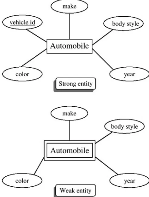
Chapt er 4 - Ext ending Relat ionships/ St ruct ural Const raint s Chapt er 5 - The Weak Ent it y
Chapt er 6 - Furt her Ext ensions for ER Diagram s w it h Binary Relat ionships Chapt er 7 - Ternary and Higher - Order ER Diagram s
Chapt er 8 - Generalizat ions and Specializat ions
Chapt er 9 - Relat ional Mapping and Reverse- Engineering ER Diagram s Chapt er 10- A Brief Overview of t he Barker/ Oracle- Like Model
Glossary I ndex
Database Design Using
Entity-Relationship Diagrams
Sikha Bagui Richard Earp
AUERBACH PUBLICATIONS
A CRC Press Company
Library of Congress Cataloging-in-Publication Data
Bagui, Sikha, 1964-
Database design using entity-relationship diagrams / Sikha Bagui, Richard Earp.
p. cm. – (Foundation of database design ; 1) Includes bibliographical references and index. 0849315484
(alk. paper)
1. Database design. 2. Relational databases. I. Earp, Richard, 1940-II. Title. III. Series.
QA76.9.D26B35 2003 005.74–dc21 2003041804
This book contains information obtained from authentic and highly regarded sources. Reprinted material is quoted with permission, and sources are indicated. A wide variety of references are listed. Reasonable efforts have been made to publish reliable data and information, but the author and the publisher cannot assume responsibility for the validity of all materials or for the consequences of their use.
Neither this book nor any part may be reproduced or transmitted in any form or by any means, electronic or mechanical, including photocopying,
microfilming, and recording, or by any information storage or retrieval system, without prior permission in writing from the publisher.
The consent of CRC Press LLC does not extend to copying for general distribution, for promotion, for creating new works, or for resale. Specific permission must be obtained in writing from CRC Press LLC for such copying.
Direct all inquiries to CRC Press LLC, 2000 N.W. Corporate Blvd., Boca Raton, Florida 33431.
Trademark Notice: Product or corporate names may be trademarks or registered trademarks, and are used only for identification and explanation, without intent to infringe.
Visit the Auerbach Web site at http://www.auerbach-publications.com
Copyright © 2003 CRC Press LLC
Auerbach is an imprint of CRC Press LLC
No claim to original U.S. Government works
International Standard Book Number 0-8493-1548-4 Library of Congress Card Number 2003041804 1 2 3 4 5 6 7 8 9 0
Dedicated to my father, Santosh Saha, and mother, Ranu Saha and
my husband, Subhash Bagui and
my sons, Sumon and Sudip and
Pradeep and Priyashi Saha
S.B.
To my wife, Brenda, and
my children: Beryl, Rich, Gen, and Mary Jo
Preface
Data modeling and database design have undergone significant evolution in recent years. Today, the relational data model and the relational database system dominate business applications. The relational model has allowed the database designer to focus on the logical and physical characteristics of a database separately. This book concentrates on techniques for database design, with a very strong bias for relational database systems, using the ER (Entity Relationships) approach for conceptual modeling (solely a logical implementation).
Intended Audience
Book Highlights
This book focuses on presenting: (1) an ER design methodology for developing an ER diagram; (2) a grammar for the ER diagrams that can be presented back to the user; and (3) mapping rules to map the ER diagram to a relational database. The steps for the ER design methodology, the grammar for the ER diagrams, as well as the mapping rules are developed and presented in a systematic, step-by-step manner throughout the book. Also, several examples of "sample data" have been included with relational database mappings — all to give a "realistic" feeling.
This book is divided into ten chapters. The first chapter gives the reader some background by introducing some relational database concepts such as functional dependencies and database normalization. The ER design method-ology and mapping rules are presented, starting in Chapter 2.
Chapter 2 introduces the concepts of the entity, attributes, relationships, and the "one-entity" ER diagram. Steps 1, 2, and 3 of the ER Design
Methodology are developed. The "one-entity" grammar and mapping rules for the" one-entity" diagram are presented.
Chapter 3 extends the one-entity diagram to include a second entity. The concept of testing attributes for entities is discussed and relationships between the entities are developed. Steps 3a, 3b, 4, 5, and 6 of the ER design methodology are developed, and grammar for the ER diagrams developed upto this point is presented.
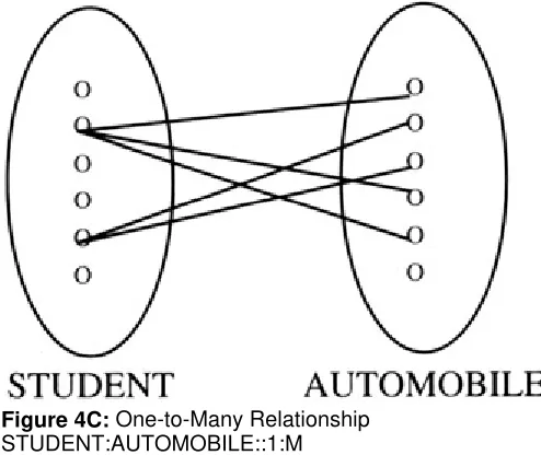
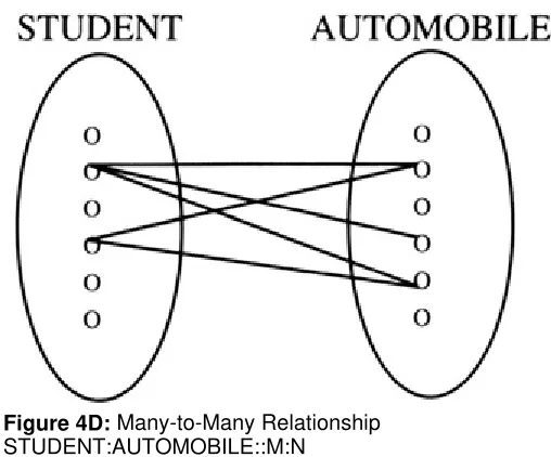
Chapter 4 discusses structural constraints in relationships. Several examples are given of 1:1, 1:M, and M:N relationships. Step 6 of the ER design
methodology is revised and step 7 is developed. A grammar for the structural constraints and the mapping rules is also presented.
Chapter 5 develops the concept of the weak entity. This chapter revisits and revises steps 3 and 4 of the ER design methodology to include the weak entity. Again, a grammar and the mapping rules for the weak entity are presented.
Chapter 6 discusses and extends different aspects of binary relationshipsin ER diagrams. This chapter revises step 5 to include the concept of more than one relationship, and revises step 6(b) to include derived and redundant relationships. The concept of the recursive relationship is introduced in this chapter. The grammar and mapping rules for recursive relationships are presented.
Chapter 7 discusses ternary and other "higher-order" relationships. Step 6 of the ER design methodology is again revised to include ternary and other, higher-order relationships. Several examples are given, and the grammar and mapping rules are developed and presented.
Chapter 8 discusses generalizations and specializations. Once again, step 6 of the ER design methodology is modified to include generalizations and specializations, and the grammar and mapping rules for generalizations and specializations are presented.
Chapter 9 provides a summary of the mapping rules and reverse-engineering from a relational database to an ER diagram.
Chapters 2 through 9 present ER diagrams using a Chen-like model.
Chapter 10 discusses the Barker/Oracle-like models, highlighting the main similarities and differences between the Chen-like model and the
Barker/Oracle-like model.
Acknowledgments
Our special thanks are due to Rich O'Hanley, President, Auerbach Publications, for his continuous support during this project. We would also like to thankGerry Jaffe, Project Editor; Shayna Murry, Cover Designer; Will Palmer, Prepress Technician, and James Yanchak, Electronic Production Manager, for their help with the production of this book.
Introduction
This book was written to aid students in database classes and to help database practitioners in understanding how to arrive at a definite, clear database design using an entity relationship (ER) diagram. In designing a database with an ER diagram, we recognize that this is but one way to arrive at the objective —the database. There are other design methodologies that also produce databases, but an ER diagram is the most common. The ER diagram (also calledan ERD) is a subset of what are called "semantic models." As we proceed through this material, we will occasionally point out where other models differ from the ER model.
The ER model is one of the best-known tools for logical database design. Within the database community it is considered to be a very natural and easy-to-understand way of conceptualizing the structure of a database. Claims that have been made for it include: (1) it is simple and easily understood by nonspecialists; (2) it is easily conceptualized, the basic constructs (entities and relationships) are highly intuitive and thus provide a very natural way of representing a user's information requirements; and (3) it is a model that describes a world in terms of entities and attributes that is most suitable for computer-naïve end users. In contrast, many educators have reported that students in database courses have difficulty grasping the concepts of the ER approach and, in particular, applying them to the real-world problems (Gold-stein and Storey, 1990).
We took the approach of starting with an entity, and then developing from it in an "inside-out strategy" (as mentioned in Elmasri and Navathe, 2000). Software engineering involves eliciting from (perhaps) "naïve" users what they would like to have stored in an information system. The process we presented follows the software engineering paradigm of
requirements/specifications, withthe ER diagram being the core of the specification. Designing a software solution depends on correct elicitation. In most software engineering paradigms, the process starts with a
requirements elicitation, followed by a specification and then a feedback loop. In plain English, the idea is (1) "tell me what you want" (requirements), and then (2) "this is what I think you want" (specification). This process of requirements/specification can (and probably should) be iterative so that users understand what they will get from thesystem and analysts will understand what the users want.
A methodology for producing an ER diagram is presented. The process leads to an ER diagram that is then translated into plain (but meant to be precise) English that a user can understand. The iterative mechanism then takes over to arrive at a specification (a revised ER diagram and English) that both users and analysts understand. The mapping of the ER diagram into arelational database is presented; mapping to other logical database models is not covered. We feel that the relational database is most appropriate to demonstrate mapping because it is the most-used
contemporary database model. Actually, the idea behind the ER diagram is to produce a high-level database model that has no particular logical model implied (relational, hierarchical, object oriented, or network).
goodness."
The approach to database design taken will be intuitive and informal.We do not deal with precise definitions of set relations. We use the
intuitive"one/many" for cardinality and "may/must" for participation
constraints. Theintent is to provide a mechanism to produce an ER diagram that can be presented to a user in English, and to polish the diagram into a specificationthat can then be mapped into a database. We then suggest testing the produced database by the theory of normal forms and other criteria (i.e., referential integrity constraints). We also suggest a reverse-mapping paradigm for reverse-mapping a relational database back to an ER diagram for the purpose of documentation.
The ER Models We Chose
We begin this venture into ER diagrams with a "Chen-like" model, and most of this book (Chapters 2 through 9) is written using the Chen-like model. Why did we choose this model? Chen (1976) introduced the idea of ER diagrams (Elmasri and Navathe, 2000), and most database texts use some variant of the Chen model. Chen and others have improved the ER process over the years; and while there is no standard ER diagram (ERD) model, the Chen-like model and variants there of are common, particularly in
comprehensive database texts. Chapter 10 briefly introduces the
"Barker/Oracle-like" model. As with the Chen model, we do not follow the Barker or Oracle models precisely, and hence we will use the term Barker/Oracle-like models in this text.
There are also other reasons for choosing the Chen-like model over the other models. With the Chen-like model, one need not consider how the database will be implemented. The Barker-like model is more intimately tied to the relational database paradigm. Oracle Corporation uses an ERD that is closer to the Barker model. Also, in the Barker-like and Oracle-like ERD, there is no accommodation for some of the features we present in the Chen-like model. For example, multi-valued attributes and weak entities are not part of the Barker or Oracle-like design process.
References
Elmasri, R. and Navathe, S.B., Fundamentals of Database Systems, 3rd ed., Addison-Wesley, Reading, MA, 2000.
Chapter 1: The Software Engineering
Process and Relational Databases
This chapter introduces some concepts that are essential to our presentation of the design of the database. We begin by introducing the idea of "software engineering" — a process of specifying systems and writing software. We then take up the subject of relational databases. Most databases in use today are relational, and the focus in this book will be to design a relational database. Before we can actually get into relational databases, we introduce the idea of functional dependencies (FDs). Once we have accepted the notion of functional dependencies, we can then easily define what is a good (and a not-so-good) database.
What Is the Software Engineering Process?
The term "software engineering" refers to a process of specifying, designing, writing, delivering, maintaining, and finally retiring software. There are many excellent references on the topic of software engineering (Schach, 1999). Some authors use the term "software engineering" synonymously with "systems analysis and design" and other titles, but the underlying point is that any information system requires some process to develop it correctly. Software engineering spans a wide range of information system problems. The problem of primary interest here is that of specifying a database. "Specifying a database" means that we will document what the database is supposed to contain.
A basic idea in software engineering is that to build software correctly, a series of steps (or phases) are required. The steps ensure that a process of thinking precedes action — thinking through "what is needed" precedes "what is written." Further, the "thinking before action" necessitates that all parties involved in software development understand and communicate with one another. One common version of presenting the thinking before acting scenario is referred to as a waterfall model (Schach, 1999), as the process is supposed to flow in a directional way without retracing.
An early step in the software engineering process involves specifying what is to be done. The waterfall model implies that once the specification of the software is written, it is not changed, but rather used as a basis for
development. One can liken the software engineering exercise to building a house. The specification is the "what do you want in your house" phase. Once agreed upon, the next step is design. As the house is designed and the blueprint is drawn, it is not acceptable to revisit the specification except for minor alterations. There has to be a meeting of the minds at the end of the specification phase to move along with the design (the blueprint) of the house to be constructed. So it is with software and database development.
Software production is a life-cycle process — it is created, used, and eventually retired. The "players" in the software development life cycle can placed into two camps, often referred to as the "user" and the "analyst." Software is designed by the analyst for the user according to the user's specification. In our presentation we will think of ourselves as the analyst trying to enunciate what the users think they want.
There is no general agreement among software engineers as to the exact number of steps or phases in the waterfall-type software development "model." Models vary, depending on the interest of the author in one part or another in the process. A very brief description of the software process goes like this:
needs.
Step 2: Specification. Write out the user wants or needs as precisely as possible.
Step 2a: Feedback the specification to the user (a review) to see if the analyst (you) have it right.
Step 2b: Re-do the specification as necessary and return to step 2a until analyst and user both understand one another and agree to move on.
Step 3: Software is designed to meet the specification from step 2.
Step 3a: Software design is independently checked against the specification and fixed until the analyst has clearly met the
specification. Note the sense of agreement in step 2 and the use of step 2 as a basis for further action. When step 3 begins, going back up the waterfall is difficult — it is supposed to be that way. Perhaps minor specification details might be revisited but the idea is to move on once each step is finished.
Step 4: Software is written (developed).
Step 4a: Software, as written, is checked against the design until the analyst has clearly met the design. Note that the specification in step 2 is long past and only minor modifications of the design would be tolerated here.
Step 5: Software is turned over to the user to be used in the application.
Step 5a: User tests and accepts or rejects until software is written correctly (it meets specification and design).
ER Diagrams and the Software Engineering Life
Cycle
This text concentrates on steps 1 through 3 of the software life cycle for database modeling. A database is a collection of related data. The concept of related data means that a database stores information about one enterprise — a business, an organization, a grouping of related people or processes. For example, a database might be about Acme Plumbing and involve customers and production. A different database might be one about the members and activities of the "Over 55 Club" in town. It would be inappropriate to have data about the "Over 55 Club" and Acme Plumbing in the same database because the two organizations are not related. Again, a database is a collection of related data.
Database systems are often modeled using an Entity Relationship (ER) diagram as the "blueprint" from which the actual data is stored — the output of the design phase. The ER diagram is an analyst's tool to diagram the data to be stored in an information system. Step 1, the requirements phase, can be quite frustrating as the analyst must elicit needs and wants from the user. The user may or may not be computer-sophisticated and may or may not know a software system's capabilities. The analyst often has a difficult time deciphering needs and wants to strike a balance of specifying something realistic.
In the real world, the "user" and the "analyst" can be committees of professionals but the idea is that users (or user groups) must convey their ideas to an analyst (or team of analysts) — users must express what they want and think they need.
User descriptions are often vague and unstructured. We will present a methodology that is designed to make the analyst's language precise enough so that the user is comfortable with the to-be-designed database, and the analyst has a tool that can be mapped directly into a database.
The early steps in the software engineering life cycle for databases would be to:
Step 1: Getting the requirements. Here, we listen and ask questions about what the user wants to store. This step often involves letting users describe how they intend to use the data that you (the analyst) will load into a database. There is often a learning curve necessary for the analyst as the user explains the system they know so well to a person who is ignorant of their specific business.
Step 2: Specifying the database. This step involves grammatical descriptions and diagrams of what the analyst thinks the user wants. Because most users are unfamiliar with the notion of an
Entity-Relationship diagram (ERD), our methodology will supplement the ERD with grammatical descriptions of what the database is supposed to contain and how the parts of the database relate to one another. The technical description of the database is often dry and uninteresting to a user; however, when analysts put what they think they heard into statements, the user and the analyst have a "meeting of the minds." For example, if the analyst makes statements such as, "All employees must generate invoices," the user may then affirm, deny, or modify the declaration to fit what is actually the case.
Step 3: Designing the database. Once the database has been diagrammed and agreed-to, the ERD becomes the blueprint for constructing the database.
1. Briefly describe the steps of the software engineering life-cycle process.
Data Models
Data must be stored in some fashion in a file for it to be useful. In database circles over the past 20 years or so, there have been three basic camps of "logical" database models — hierarchical, network, and relational — three ways of logically perceiving the arrangement of data in the file structure. This section provides some insight into each of these three main models along with a brief introduction to the relational model.
The Hierarchical Model
The idea in hierarchical models is that all data is arranged in a hierarchical fashion (a.k.a. a parent–child relationship). If, for example, we had a database for a company and there was an employee who had dependents, then one would think of an employee as the "parent" of the dependent. (Note: Understand that the parent–child relationship is not meant to be a human relationship. The term "parent–child" is simply a convenient reference to a common familial relationship. The "child" here could be a dependent spouse or any other human relationship.) We could have every dependent with one employee parent and every employee might have multiple dependent children. In a database, information is organized into files, records, and fields. Imagine a file cabinet we call the employee file: it contains all information about employees of the company. Each employee has an employee record, so the employee file consists of individual
employee records. Each record in the file would be expected to be organized in a similar way. For example, you would expect that the person's name would be in the same place in each record. Similarly, you would expect that the address, phone number, etc. would be found in the same place in everyone's records. We call the name a "field" in a record. Similarly, the address, phone number, salary, date of hire, etc. are also fields in the employee's record. You can imagine that a parent (employee) record might contain all sorts of fields — different companies have different needs and no two companies are exactly alike.
In addition to the employee record, we will suppose in this example that the company also has a dependent file with dependent information in it — perhaps the dependent's name, date of birth, place of birth, school attending, insurance information, etc. Now imagine that you have two file cabinets: one for employees and one for dependents. The connection between the records in the different file cabinets is called a "relationship." Each dependent must be related to some employee, and each employee may or may not have a dependent in the dependent file cabinet.
Relationships in all database models have what are called "structural constraints." A structural constraint consists of two notions: cardinality and optionality. Cardinality is a description of how many of one record type relate to the other, and vice versa. In our company, if an employee can have multiple dependents and the dependent can have only one employee parent, we would say the relationship is one-to-many — that is, one employee, many dependents. If the company is such that employees might have multiple dependents and a dependent might be claimed by more that one employee, then the cardinality would be many-to-many — many employees, many dependents. Optionality refers to whether or not one record may or must have a corresponding record in the other file. If the employee may or may not have dependents, then the optionality of the employee to dependent relationship is "optional" or "partial." If the dependents must be "related to" employee(s), then the optionality of dependent to employee is "mandatory" or "full."
description. We could say that:
Employees may have zero or more dependents
and
Dependents must be associated with one and only one employee.
Note the employee-to-dependent, one-to-many cardinality and the optional/mandatory nature of the relationship.
All relationships between records in a hierarchical model have a cardinality of one-to-many or one-to-one, but never many-to-one or many-to-many. So, for a hierarchical model of employee and dependent, we can only have the employee-to-dependent relationship as one-to-many or one-to-one; an employee may have zero or more dependents, or (unusual as it might be) an employee may have one and only one dependent. In the hierarchical model, you could not have dependents with multiple parent–employees.
The original way hierarchical databases were implemented involved choosing some way of physically "connecting" the parent and the child records. Imagine you have looked up an employee in the employee filing cabinet and you want to find the dependent records for that employee in the dependent filing cabinet. One way to implement the employee–dependent relationship would be to have an employee record point to a dependent record and have that dependent record point to the next dependent (a linked list of child –records, if you will). For example, you find employee Jones. In Jones' record, there is a notation that Jones' first dependent is found in the dependent filing cabinet, file drawer 2, record 17. The "file drawer 2, record 17" is called a pointer and is the "connection" or "relationship" between the employee and the dependent. Now to take this example further, suppose the record of the dependent in file drawer 2, record 17 points to the next
dependent in file drawer 3, record 38; then that person points to the next dependent in file drawer 1, record 82.
In the linked list approach to connecting parent and child records, there are advantages and disadvantages to that system. For example, one advantage would be that each employee has to maintain only one pointer and that the size of the "linked list" of dependents is theoretically unbounded. Drawbacks would include the fragility of the system in that if one dependent record is destroyed, then the chain is broken. Further, if you wanted information about only one of the child records, you might have to look through many records before you find the one you are looking for.
There are, of course, several other ways of making the parent–child link. Each method has advantages and disadvantages, but imagine the difficulty with the linked list system if you wanted to have multiple parents for each child record. Also note that some system must be chosen to be implemented in the underlying database software. Once the linking system is chosen, it is fixed by the software implementation; the way the link is done has to be used to link all child records to parents, regardless of how inefficient it might be for one situation.
There are three major drawbacks to the hierarchical model:
1. Not all situations fall into the one-to-many, parent–child format.
2. The choice of the way in which the files are linked impacts performance, both positively and negatively.
dependent file were reorganized, then all pointers would have to be reset.
The Network Model
The network model was developed as a successor to the hierarchical model. The network model alleviated the first concern as in the network model — one was not restricted to having one parent per child — a many-to-many relationship or a many-to-one relationship was acceptable. For example, suppose that our database consisted of our employee–dependent situation as in the hierarchical model, plus we had another relationship that involved a "school attended" by the dependent. In this case, the employee–dependent relationship might still be one-to-many, but the "school attended"–dependent relationship might well be many-to-many. A dependent could have two "parent/schools." To implement the dependent–school relationship in hierarchical databases involved creating redundant files, because for each school, you would have to list all dependents. Then, each dependent who attended more than one school would be listed twice or three times, once for each school. In network databases we could simply have two connections or links from the dependent child to each school, and vice versa.
The second and third drawbacks of hierarchical databases spilled over to network databases. If one were to write a database system, one would have to choose some method of physically connecting or linking records. This choice of record connection then locks us into the same problem as before, a hardware-implemented connection that impacts performance both positively and negatively. Further, as the database becomes more complicated, the paths of connections and the maintenance problems become exponentially more difficult to manage.
The Relational Model
E. Codd (ca. 1970) introduced the relational model to describe a database that did not suffer from the drawbacks of the hierarchical and network models. Codd's premise was that if we ignore the way data files are connected and arrange our data into simple two-dimensional, unordered tables, then we can develop a calculus for queries (questions posed to the database) and focus on the data as data, not as a physical realization of a logical model. Codd's idea was truly logical in that one was no longer concerned with how data was physically stored. Rather, data sets were simply unordered, two-dimensional tables of data. To arrive at a workable way of deciding which pieces of data went into which table, Codd proposed "normal forms." To understand normal forms, we must first introduce the notion of "functional dependencies." After we understand functional dependences, the normal forms follow.
Checkpoint 1.2
1. What are the three main types of data models?
2. Which data model is mostly used today? Why?
3. What are some of the disadvantages of the hierarchical data model?
4. What are some of the disadvantages of the network data model?
5. How are all relationships (mainly the cardinalities) described in the hierarchical data model? How can these be a disadvantage of the hierarchical data model?
network data model? Would you treat these as advantages or disadvantages of the network data model? Discuss.
Functional Dependencies
A functional dependency is a relationship of one attribute or field in a record to another. In a database, we often have the case where one field defines
the other. For example, we can say that Social Security Number (SSN) defines a name. What does this mean? It means that if I have a database with SSNs and names, and if I know someone's SSN, then I can find their name. Further, because we used the word "defines," we are saying that for every SSN we will have one and only one name. We will say that we have
defined name as being functionally dependent on SSN.
The idea of a functional dependency is to define one field as an anchor from which one can always find a single value for another field. As another example, suppose that a company assigned each employee a unique employee number. Each employee has a number and a name. Names might be the same for two different employees, but their employee numbers would always be different and unique because the company defined them that way. It would be inconsistent in the database if there were two occurrences of the same employee number with different names.
We write a functional dependency (FD) connection with an arrow:
SSN → Name
or
EmpNo → Name.
The expression SSN→Name is read "SSN defines Name" or "SSN implies Name."
Let us look at some sample data for the second FD.
Wait a minute…. You have two people named Fred! Is this a problem with FDs? Not at all. You expect that Name will not be unique and it is
commonplace for two people to have the same name. However, no two people have the same EmpNo and for each EmpNo, there is a Name.
Let us look at a more interesting example:
EmpNo Name 101 Kaitlyn 102 Brenda 103 Beryl 104 Fred 105 Fred
EmpNo Job Name
101 President Kaitlyn
104 Programmer Fred 103 Designer Beryl
Is there a problem here? No. We have the FD that EmpNo→Name. This means that every time we find 104, we find the name, Fred. Just because something is on the left-hand side (LHS) of a FD, it does not imply that you have a key or that it will be unique in the database — the FD X→Y only means that for every occurrence of X you will get the same value of Y.
Let us now consider a new functional dependency in our example. Suppose that Job→Salary. In this database, everyone who holds a job title has the same salary. Again, adding an attribute to the previous example, we might see this:
Do we see a contradiction to our known FDs? No. Every time we find an
EmpNo, we find the same Name; every time we find a Job title, we find the same Salary.
Let us now consider another example. We will go back to the SSN→Name
example and add a couple more attributes.
Here, we will define two FDs: SSN→Name and School→Location.
Further, we will define this FD: SSN→School.
First, have we violated any FDs with our data? Because all SSNs are unique, there cannot be a FD violation of SSN→Name. Why? Because a FD X→Y
says that given some value for X, you always get the same Y. Because the
X's are unique, you will always get the same value. The same comment is true for SSN→School.
EmpNo Job Name Salary
101 President Kaitlyn 50 104 Programmer Fred 30
103 Designer Beryl 35 103 Programmer Beryl 30
SSN Name School Location
101 David Alabama Tuscaloosa
102 Chrissy MSU Starkville
103 Kaitlyn LSU Baton Rouge 104 Stephanie MSU Starkville
How about our second FD, School→Location? There are only three schools in the example and you may note that for every school, there is only one location, so no FD violation.
Now, we want to point out something interesting. If we define a functional dependency X→Y and we define a functional dependency Y→Z, then we
know by inference that X→Z. Here, we defined SSN→School. We also
defined School→Location, so we can infer that SSN→Location
although that FD was not originally mentioned. The inference we have illustrated is called the transitivity rule of FD inference. Here is the transitivity rule restated:
Given X → Y
Given Y → Z
Then X → Z
To see that the FD SSN→Location is true in our data, you can note that given any value of SSN, you always find a unique location for that person. Another way to demonstrate that the transitivity rule is true is to try to invent a row where it is not true and then see if you violate any of the defined FDs.
We defined these FD's:
Given: SSN → Name
SSN → School
School → Location
We are claiming by inference using the transitivity rule that SSN→
Location. Suppose that we add another row with the same SSN and try a different location:
Now, we have satisfied SSN→Name but violated SSN→Location. Can we do this? We have no value for School, but we know that if School = "Alabama" as defined by SSN→School, then we would have the following rows:
SSN Name School Location
101 David Alabama Tuscaloosa
102 Chrissy MSU Starkville
103 Kaitlyn LSU Baton Rouge 104 Stephanie MSU Starkville
105 Lindsay Alabama Tuscaloosa 106 Chloe Alabama Tuscaloosa
However, this is a problem. We cannot have Alabama and Starkville in the same row because we also defined School→Location. So in creating our counterexample, we came upon a contradiction to our defined FDs. Hence, the row with Alabama and Starkville is bogus. If you had tried to create a new location like this:
You violate the FD, SSN→School — again, a bogus row was created. By being unable to provide a counterexample, you have demonstrated that the transitivity rule holds. You may prove the transitivity rule more formally (see Elmasri and Navathe, 2000, p. 479).
There are other inference rules for functional dependencies. We will state them and give an example, leaving formal proofs to the interested reader (see Elmasri and Navathe, 2000).
The Reflexive Rule
If X is a composite, composed of A and B, then X→A and X→B. Example: X
= Name, City. Then we are saying that X→Name and X→City.
Example:
The rule, which seems quite obvious, says if I give you the combination
<Kaitlyn, New Orleans>, what is this person's Name? What is this person's City? While this rule seems obvious enough, it is necessary to derive other functional dependencies.
The Augmentation Rule
If X→Y, then XZ→Y. You might call this rule, "more information is not really needed, but it doesn't hurt." Suppose we use the same data as before with Names and Cities, and define the FD Name→City. Now, suppose we add a column, Shoe Size:
SSN Name School Location
106 Chloe Alabama Tuscaloosa 106 Chloe Alabama Starkville
SSN Name School Location
106 Chloe Alabama Tuscaloosa
106 Chloe FSU Tallahassee
Name City
David Mobile Kaitlyn New Orleans
Now, I claim that because Name→City, that Name+Shoe Size→City
(i.e., we augmented Name with Shoe Size). Will there be a contradiction here, ever? No, because we defined Name→City, Name plus more information will always identify the unique City for that individual. We can always add information to the LHS of an FD and still have the FD be true.
The Decomposition Rule
The decomposition rule says that if it is given that X→YZ (that is, X defines
both Y and Z), then X→Y and X→Z. Again, an example:
Suppose I define Name→City, Shoe Size. This means for every occurrence of Name, I have a unique value of City and a unique value of
Shoe Size. The rule says that given Name→City and Shoe Size
together, then Name→City and Name→Shoe Size. A partial proof using the reflexive rule would be:
Name → City, Shoe Size (given)
City, Shoe Size → City (by the reflexive rule)
Name → City (using steps 1 and 2 and the transitivity rule)
The Union Rule
The union rule is the reverse of the decomposition rule in that if X→Y and X
→Z, then X→YZ. The same example of Name, City, and Shoe Size
illustrates the rule. If we found independently or were given that Name→
City and given that Name→Show Size, we can immediately write Name
→City, Shoe Size. (Again, for further proofs, see Elmasri and Navathe, 2000, p. 480.)
You might be a little troubled with this example in that you may say that
Name is not a reliable way of identifying City; Names might not be unique. You are correct in that Names may not ordinarily be unique, but note the
Name City Shoe Size
David Mobile 10
Kaitlyn New Orleans 6
Chrissy Baton Rouge 3
Name City Shoe Size
David Mobile 10
Kaitlyn New Orleans 6
language we are using. In this database, we define that Name→City and, hence, in this database are restricting Name to be unique by definition.
Keys and FDs
The main reason we identify the FDs and inference rules is to be able to find keys and develop normal forms for relational databases. In any relational table, we want to find out which, if any attribute(s), will identify the rest of the attributes. An attribute that will identify all the other attributes in row is called a "candidate key." A "key" means a "unique identifier" for a row of
information. Hence, if an attribute or some combination of attributes will always identify all the other attributes in a row, it is a "candidate" to be "named" a key. To give an example, consider the following:
Now suppose I define the following FDs:
SSN → Name
SSN → School
School → Location
What I want is the fewest number of attributes I can find to identify all the rest — hopefully only one attribute. I know that SSN looks like a candidate, but can I rely on SSN to identify all the attributes? Put another way, can I show that SSN "defines" all attributes in the relation? I know that SSN defines Name and School because that is given. I know that I have the following transitive set of FDs:
SSN → School
School → Location
Therefore, by the transitive rule, I can say that SSN→Location. I have derived the three FDs I need. Adding the reflexive rule, I can then use the union rule:
SSN → Name (given)
SSN → School (given)
SSN → Location (derived by the transitive rule)
SSN → SSN (reflexive rule (obvious))
SSN → SSN, Name, School, Location (union rule)
SSN Name School Location
101 David Alabama Tuscaloosa
102 Chrissy MSU Starkville 103 Kaitlyn LSU Baton Rouge
104 Stephanie MSU Starkville
This says that given any SSN, I can find a unique value for each of the other fields for that SSN. SSN therefore is a candidate key for this relation. In FD theory, once we find all the FDs that an attribute defines, we have found the
closure of the attribute(s). In our example, the closure of SSN is all the attributes in the relation. Finding a candidate key is the finding of a closure of an attribute or a set of attributes that defines all the other attributes.
Are there any other candidate keys? Of course! Remember the
augmentation rule that tells us that because we have established the SSN as the key, we can augment SSN and form new candidate keys: SSN, Name is a candidate key. SSN, Location is a candidate key, etc. Because every row in a relation is unique, we always have at least one candidate key — the set of all the attributes.
Is School a candidate key? No. You do have the one FD that School→
Location and you could work on this a bit, but you have no way to infer that School→SSN (and in fact with the data, you have a counterexample that shows that School does not define SSN).
Keys should be a minimal set of attributes whose closure is all the attributes in the relation — "minimal" in the sense that you want the fewest attributes on the LHS of the FD that you choose as a key. In our example, SSN will be minimal (one attribute), whose closure includes all the other attributes.
Once we have found a set of candidate keys (or perhaps only one as in this case), we designate one of the candidate keys as the primary key and move on to normal forms.
These FD rules are useful in developing Normal forms. Normal forms can be expressed in more than one way, but using FDs is arguably the easiest way to see this most fundamental relational database concept. E. Codd (1972) originally defined three normal forms: 1NF, 2NF, and 3NF.
Checkpoint 1.3
1. What are functional dependencies? Give examples.
2. What does the augmentative rule state? Give examples.
A Brief Look at Normal Forms
In this section we briefly describe the first, second, and third normal forms.
First Normal Form (1NF)
The first normal form (1NF) requires that data in tables be two-dimensional — that there be no repeating groups in the rows. An example of a table not in 1NF is where there is an employee "record" such as:
Employee(name, address, {dependent name})
where {dependent name} infers that the attribute is repeated. Sample data for this record might be:
Smith, 123 4th St., {John, Mary, Paul, Sally} Jones, 4 Moose Lane., {Edgar, Frank, Bob}
Adams, 88 Tiger Circle., {Kaitlyn, Alicia, Allison}
The problem with putting data in tables with repeating groups is that the table cannot be easily indexed or arranged so that the information in the repeating group can be found without searching each record individually. Relational people usually call a repeating group "nonatomic" (it has more than one value and can be broken apart).
Second Normal Form (2NF)
The second normal form (2NF) requires that data in tables depends on the whole key of the table. Partial dependencies are not allowed. An example:
Employee (name, job, salary, address)
where it takes a name + job combination (a concatenated key) to identify a
salary, but address depends only on name. Some sample data:
Can you see the problem developing here? The address would be repeated for each occurrence of a name. This repeating is called redundancy and leads to anomalies. An anomaly means that there is a restriction on doing something due to the arrangement of the data. There are insertion
anomalies, deletion anomalies, and update anomalies. The key of this table is Name + Job — this is clear because neither one is unique and it really takes both name and job to identify a salary. However, address depends only on the name, not the job; this is an example of a partial dependency.
Address depends on only part of the key. An example of an insertion anomaly would be where one would want to insert a person into the table above, but the person to be inserted is not yet assigned a job. This cannot be done because a value would have to be known for the job attribute. Null
Name Job Salary Address
Smith Welder 14.75 123 4th St Smith Programmer 24.50 123 4th St
Smith Waiter 7.50 123 4th St
Jones Programmer 26.50 4 Moose Lane Jones Bricklayer 34.50 4 Moose Lane
values cannot be valid values for keys in relational databases (this is known as the entity-integrity constraint). An update anomaly would be where one of the employees changed his or her address. Three rows would have to be changed to accommodate this one change of address. An example of a delete anomaly would be that Adams quits, so Adams is lost, but then the information that the analyst is being paid $28.50 is also lost. Therefore, more related information than was previously anticipated is lost.
Third Normal Form (3NF)
The third normal form (3NF) requires that the data in tables depends on the primary key of the table. A classic example of non-3NF is:
Employee (name, address, project#, project-location)
Suppose that project-location means the location from which a project is controlled, and is defined by the project#. Some sample data will show the problem with this table:
Note the redundancy in this table. Project 101 is located in Memphis; but every time a person is recorded as working on project 101, the fact that they work on a project that is controlled from Memphis is recorded again. The same anomalies — insert anomaly, update anomaly, and delete anomaly — are also present in this table.
To clear the database of anomalies and redundancies, databases must be normalized. The normalization process involves splitting the table into two or more tables (a decomposition). After tables are split apart (a process called decomposition), they can be reunited with an operation called a "join." There are three decompositions that would alleviate the normalization problems in our examples, as discussed below.
Examples of 1NF, 2NF, and 3NF
Example of Non-1NF to 1NF
Here, the repeating group is moved to a new table with the key of the table from which it came.
Non-1NF:
Smith, 123 4th St., {John, Mary, Paul, Sally} Jones, 4 Moose Lane., {Edgar, Frank, Bob}
Adams, 88 Tiger Circle., {Kaitlyn, Alicia, Allison}
is decomposed into 1NF tables with no repeating groups:
1NF Tables:
Name Address Project# Project-location
Smith 123 4th St 101 Memphis
Smith 123 4th St 102 Mobile Jones 4 Moose Lane 101 Memphis
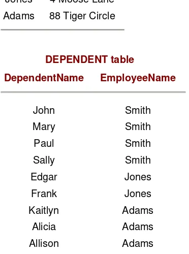
EMPLOYEE table
In the EMPLOYEE table, Name is defined as a key — it uniquely identifies the rows. In the DEPENDENT table, the key is a combination
(concatenation) of DependentName and EmployeeName. Neither the
DependentName nor the EmployeeName is unique in the DEPENDENT
table, and therefore both attributes are required to uniquely identify a row in the table. The EmployeeName in the DEPENDENT table is called a foreign key because it references a primary key, Name in another table, the
EMPLOYEE table. Note that the original table could be reconstructed by combining these two tables by recording all the rows in the EMPLOYEE table and combining them with the corresponding rows in the EMPLOYEE table where the names were equal (an equi-join operation). Note that in the derived tables, there are no anomalies or unnecessary redundancies.
Example of Non-2NF to 2NF
Here, partial dependency is removed to a new table.
Non-2NF:
Smith 123 4th St Jones 4 Moose Lane
Adams 88 Tiger Circle
DEPENDENT table
DependentName EmployeeName
John Smith
Mary Smith Paul Smith
Sally Smith
Edgar Jones Frank Jones
Kaitlyn Adams
Alicia Adams Allison Adams
Name Job Salary Address
Smith Welder 14.75 123 4th St
Smith Programmer 24.50 123 4th St Smith Waiter 7.50 123 4th St
Jones Programmer 26.50 4 Moose Lane
is decomposed into 2NF:
Name + Job table
Name and Address (Employee info) table:
Again, note the removal of unnecessary redundancy and the amelioration removal of possible anomalies.
Example of Non-3NF to 3NF
Here, transitive dependency is removed to a new table.
Non-3NF:
is decomposed into 3NF:
EMPLOYEE table:
NAME AND JOB
Name Job Salary
Smith Welder 14.75
Smith Programmer 24.50 Smith Waiter 7.50
Jones Programmer 26.50
Jones Bricklayer 34.50 Adams Analyst 28.50
NAME AND ADDRESS
Name Address
Smith 123 4th St Jones 4 Moose Lane
Adams 88 Tiger Circle
Name Address Project# Project-location
Smith 123 4th St 101 Memphis
Smith 123 4th St 102 Mobile
Jones 4 Moose Lane 101 Memphis
EMPLOYEE
Name Address Project#
PROJECT table:
Again observe the removal of the transitive dependency and the anomaly problem.
There are more esoteric normal forms, but most databases will be well constructed if they are normalized to the 3NF. The intent here is to show the general process and merits of normalization.
Checkpoint 1.4
1. Define 1NF, 2NF, and 3NF.
2. Why do databases have to be normalized?
3. Why should we avoid having attributes with multiple values or repeating groups?
Smith 123 4th St 102
Jones 4 Moose Lane 101
PROJECT
Project# Project-location
101 Memphis
102 Mobile
Chapter Summary
Chapter 1 Exercises
Example 1.1
If X→Y, can you say Y→X? Why or why not ?
Example 1.2
Decompose the following data into 1NF tables:
Khanna, 123 4th St., Columbus, Ohio {Delhi University, Calcutta University, Ohio State}
Ray, 4 Moose Lane, Pensacola, Florida {Zambia University, University of West Florida}
Ali, 88 Tiger Circle, Gulf Breeze, Florida {University of South Alabama, University of West Florida}
Sahni, 283 Penny Street, North Canton, Ohio {Wooster College, Mount Union College}
Example 1.3
Does the following data have to be decomposed?
Name Address City State Car Color Year
Smith 123 4th St.
Pensacola FL Mazda Blue 2002
Smith 123 4th St.
Pensacola FL Nissan Red 2001
Jones 4 Moose Lane
Santa Clive
CA Lexus Red 2000
Katie 5 Rain Circle
Fort Walton
References
Armstrong, W. "Dependency Structures of Data Base Relationships," Proceedings of the IFIP Congress, 1974.
Chen, P.P. "The Entity Relationship Model — Toward a Unified View of Data,"ACM TODS 1, No. 1, March 1976.
Codd, E. "A Relational Model for Large Shared Data Banks,"CACM, 13, 6, June 1970.
Codd, E. Further Normalization of the Data Base Relational Model, in Rustin (1972).
Codd, E. "Recent Investigations in Relational Database System," Proceedings of the IFIP Congress, 1974.
Date, C. An Introduction to Database Systems, 6th ed., Addison-Wesley, Reading, MA, 1995.
Elmasri, R. and Navathe, S.B. Fundamentals of Database Systems, 3rd ed., Addison-Wesley, Reading, MA, 2000.
Maier, D. The Theory of Relational Databases, Computer Science Press, Rockville, MD, 1983.
Norman, R.J. Object-Oriented Systems Analysis and Design, Prentice Hall, Upper Saddle River, NJ, 1996.
Chapter 2: The Basic ER Diagram—A
Data Modeling Schema
This chapter begins by describing a data modeling approach and then introduces entity relationship (ER) diagrams. The concept of entities, attributes, relationships, and keys are introduced. The first three steps in an ER design methodology are developed. Step 1 begins by building a one-entity diagram. Step 2 concentrates on using structured English to describe a database. Step 3, the last section in this chapter, discusses mapping the ER diagram to a relational database. These concepts — the diagram, structured English, and mapping — will evolve together as the book progresses. At the end of the chapter we also begin a running case study, which will be continued at the ends of the subsequent chapters.
What Is a Data Modeling Schema?
A data modeling schema is a method that allows us to model or illustrate a database. This device is often in the form of a graphic diagram, but other means of communication are also desirable — non computer-people may or may not understand diagrams and graphics. The ER diagram (ERD) is a graphic tool that facilitates data modeling. The ERD is a subset of "semantic models" in a database. Semantic models refer to models that intend to elicit meaning from data. ERDs are not the only semantic modeling tools, but they are common and popular.
When we begin to discuss the contents of a database, the data model helps to decide which piece of data goes with which other piece of data on a conceptual level. An early concept in databases is to recognize that there are levels of abstraction that we can use in discussing databases. For example, if we were to discuss the filing of "names," we could discuss this:
Abstractly, that is, "we will file names of people we know."
or
Concretely, that is, "we will file first, middle, and last names (20 characters each) of people we know, so that we can retrieve the names in alphabetical order on last name, and we will put this data in a spreadsheet format on package x."
If a person is designing a database, the first step is to abstract and then refine the abstraction. The longer one stays away from the concrete details of logical models (relational, hierarchical, network) and physical realizations (fields [how many characters, the data type, etc.] and files [relative,
spreadsheet]), the easier it is to change the model and to decide how the data will eventually be physically realized (stored). When we use the term "field" or "file," we will be referring to physical data as opposed to conceptual data.
Mapping is the process of choosing a logical model and then moving to a physical database file system from a conceptual model (the ER diagram). A physical file loaded with data is necessary to actually get data from a database. Mapping is the bridge between the design concept and physical reality. In this book we concentrate on the relational database model due to its ubiquitousness in contemporary database models.
The ER diagram is a semantic data modeling tool that is used to accomplish the goal of abstractly describing or portraying data. Abstractly described data is called a conceptual model. Our conceptual model will lead us to a "schema." A schema implies a permanent, fixed description of the structure of the data. Therefore, when we agree that we have captured the correct depiction of reality within our conceptual model, our ER diagram, we can call it a schema.
Defining the Database — Some Definitions: Entity,
Relationship, Attribute
As the name implies, an ER diagram models data as entities and
relationships, and entities have attributes. An entity is a thing about which we store data, for example, a person, a bank account, a building. In the original presentation, Chen (1976) described an entity as a "thing which can be distinctly identified." So an entity can be a person, place, object, event, or concept about which we wish to store data.
The name for an entity must be one that represents a type or class of thing, not an instance. The name for an entity must be sufficiently generic but, at the same time, the name for an entity cannot be too generic. The name should also be able to accommodate changes "over time." For example, if we were modeling a business and the business made donuts, we might consider creating an entity called DONUT. But how long will it be before this business evolves into making more generic pastry? If it is anticipated that the business will involve pastry of all kinds rather than just donuts, perhaps it would be better to create an entity called PASTRY — it may be more applicable "over time."
Some examples of entities include:
Examples of a person entity would be EMPLOYEE, VET, or STUDENT.
Examples of a place entity would be STATE or COUNTRY.
Examples of an object entity would be BUILDING, AUTO, or PRODUCT.
Example of an event entity would be SALES, RETURNS, or REGISTRATION.
Examples of a concept entity would be ACCOUNT or DEPARTMENT.
In older data processing circles, we might have referred to an entity as a record, but the term "record" is too physical and too confining; "record" gives us a mental picture of a physical thing and, in order to work at the conceptual level, we want to avoid device-oriented pictures for the moment. In a
database context, it is unusual to store information about one entity, so we think of storing collections of data about entities — such collections are called entity sets. Entity sets correspond to the concept of "files," but again, a file usually connotes a physical entity and hence we abstract the concept of the "file" (entity set) as well as the concept of a "record" (entity). As an example, suppose we have a company that has customers. You would imagine that the company had a customer entity set with individual customer entities in it.
An entity may be very broad (e.g., a person), or it may be narrowed by the application for which data is being prepared (like a student or a customer).
Broad entities, which cover a whole class of objects, are sometimes called generalizations (e.g., person), and narrower entities are sometimes called specializations (e.g., student). In later diagrams (in this book) we will revisit generalizations and specializations; but for now, we will concern ourselves with an application level where there are no subgroups (specializations) or supergroups (generalizations) of entities.
When we speak of capturing data about a particular entity, we refer to this as an instance. An entity instance is a single occurrence of an entity. For example, if we create an entity called TOOL, and if we choose to record data about a screwdriver, then the screwdriver "record" is an instance of TOOL. Each instance of an entity must be uniquely identifiable so that each
type of entity. In a customer entity set, you might imagine that the company would assign a unique customer number, for example. This unique identifier is called a key.
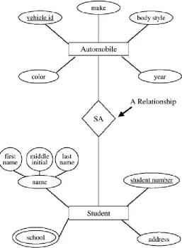
A relationship is a link or association between entities. Relationships are usually denoted by verb phrases. We will begin by expanding the notion of an entity (in this chapter and the next), and then we will come back to the notion of a relationship (in Chapter 4) once we have established the concept of an entity.
A Beginning Methodology
Database modeling begins with a description of "what is to be stored." Such a description can come from anyone; we will call the describer the "user." For example, Ms. Smith of Acme Parts Company comes to you, asking that you design a database of parts for her company. Ms. Smith is the user. You are the database designer. What Ms. Smith tells you about the parts will be the database description.
As a starting point in dealing with a to-be-created database we will identify a central, "primary" entity — a category about which we will store data. For example, if we wanted to create a database about students and their
environment, then one entity would be STUDENT (our characterization of an entity will always be in the singular). Having chosen one first primary entity, STUDENT, we will then search for information to be recorded about our STUDENT. This methodology of selecting one "primary" entity from a data description is our first step in drawing an ER diagram, and hence the beginning of the requirements phase of software engineering for our database.
Once the "primary" entity has been chosen, we then ask ourselves what information we want to record about our entity. In our STUDENT example, we add some details about the STUDENT — any details that will qualify, identify, classify, or express the state of the entity (in this case, the
STUDENT entity). These details or contents of entities are called attributes.
[1] Some example attributes of STUDENT would be the student's name,
student number, major, address, etc. — information about the student.
[1]C. Date (1995) prefers the word "property" to "attribute" because it is more
ER Design Methodology
Step 1: Select one primary entity from the database requirements description and show attributes to be recorded for that entity.
"Requirements definition" is the first phase of software engineering where the systems analyst tries to find out what a user wants. In the case of a database, an information-oriented system, the user will want to store data. Now that we have chosen a primary entity and some attributes, our task will be to:
Draw a diagram of our first-impression entity (our primary entity).
Translate the diagram into English.
Present the English (and the diagram) back to the user to see if we have it right and then progress from there.
The third step is called "feedback" in software engineering. The process of refining via feedback is a normal process in the requirements/specification phases. The feedback loop is essential in arriving at the reality of what one wants to depict from both the user and analyst viewpoints. First we will learn how to draw the entity and then we will present guidelines for converting our diagram into English.
Checkpoint 2.1
1. Of the following items, determine which could be an entity and state why: automobile, college class, student, name of student, book title, number of dependents.
2. Why are entities not called files or records?
3. What is mapping?
4. What are entity sets?
5. Why do we need Entity-Relationship Diagrams?
6. What are attributes? List attributes of the entities you found in question 1 (above).
A First "Entity-Only" ER Diagram: An Entity with
Attributes
To recap our example, we have chosen an example with a "primary" entity from a student information database — the student. Again note that "a student" is something about which we want to store information (the
definition of an entity). In this chapter, we do not concern ourselves with any other entities.
Let us think about some attributes of the entity STUDENT; that is, what are some attributes a student might have? A student has a name, an address, and an educational connection. We will call the educational connection a "school." We have picked three attributes for the entity STUDENT, and we have also chosen a generic label for each: name, address, school.
We begin our first venture into ER diagrams with a "Chen-like" model. Chen (1976) introduced the idea of the ER diagrams. He and others have
improved the ER process over the years; and while there is no standard ERD model, the Chen-like model and variants thereof are common. After the "Chen-like" model, we introduce other models. We briefly discuss the "Barker/Oraclelike" model later (in Chapter 10). Chen-like models have the advantage that one does not need to know the underlying logical model to understand the design. Barker models and some other models require a full understanding of the relational model, and the diagrams are affected by relational concepts.
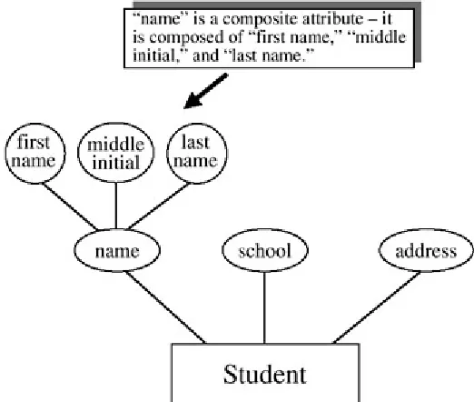
To begin, in the Chen-like model, we will do as Chen originally did and put the entities in boxes and the show attributes nearby. One way to depict attributes is to put them in circles or ovals appended to the boxes — see
Figure 2.1: An ER Diagram with Three Attributes
Figure 2.2: An ER Diagram with One Entity and Five Attributes, Alternate Models (Batini, Ceri, Navathe)
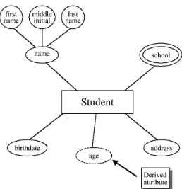
Figure 2.1 (middle and bottom) shows an ER diagram with one entity, STUDENT, and three attributes: name, address, and school. If more attributes are added to our conceptual model, such as phone and major, they would be appended to the entity (here, STUDENT is the only entity we have), as can be seen in Figure 2.3.
More about Attributes
Attributes are characteristics of entities that provide descriptive details about the entities. There are several different kinds of attributes: simple or atomic, composite, multi-valued, and derived. The properties of an attribute are its name, description, format, and length, in addition to its atomiticity. Some attributes may be considered unique identifiers for an entity. This section also introduces the idea of a key attribute, a unique identifier for an entity.
The Simple or Atomic Attribute
Simple or atomic attributes cannot be further broken down or subdivided, hence the notion "atomic." One can examine the domain of values[2] of an
attribute to elicit whether an attribute is simple or not. An example of a simple or atomic attribute would be Social Security number, where a person would be expected to have only one, undivided Social Security number.
Other tests of whether an attribute is simple or atomic will depend entirely on the circumstances that the database designer encounters — the desire of the "user" for which the database is being built. For example, we might treat a phone number attribute as simple in a particular database design, but in another scenario we may want to divide the phone number into two distinct parts, that is, the area code and the number. Another example of where the use of the attribute in the database will determine if the attribute is simple or atomic is — a birthdate attribute. If we are setting up a database for a veterinary hospital, it may make sense to break up a birthdate field into month, day, and year, because it will make a difference in treatment if a young animal is five days old versus if it is five months or five years old. Hence, in this case, birthdate would be a composite attribute. For a RACE HORSE database, however, it may not be necessary to break up a birthdate field into month/day/year, because all horses are dated only by the year in which they were born. In this latter case, birthdate, consisting of only the year, would be atomic.
If an attribute is non-atomic, it needs to be depicted as such on the ER diagram. The following sections deal with these more complicated, nonatomic attribute ideas — the composite attribute and the multi-valued attribute.
The Composite Attribute
A composite attribute, sometimes called a group attribute, is an attribute formed by combining or aggregating related attributes. The names chosen for composite attributes should be descriptive and general. The concept of "name" is adequate for a general description, but it may be desirable to be more specific about the parts of this attribute. Most data processing applications divide the name into component parts. Name, then, is called a
composite attribute or an aggregate because it is usually composed of a first name, a last name, and a middle initial — sub-attributes, if you will. The way that composite attributes are shown in ER diagrams in the Chen-like model is illustrated in Figure 2.4. The sub-attributes, such as first name, middle initial, and last name, are called simple, atomic, or elementary
Figure 2.4: An ER Diagram with a Composite Attribute —
name
Once again, the test of whether or not an attribute will be composite will depend entirely on the circumstances that the database designer encounters — the desire of the "user" for which the database is being built. For example, in one database it may not be important to know exactly which city or state or zip code a person comes from, so an address attribute in that database may not be broken up into its component parts; it may just be called address. Whereas in another database, it may be important to know which city and state a person is from; so in this second database we would have to break up the address attribute into street address, city, state, and zip code, making the address attribute a composite attribute.
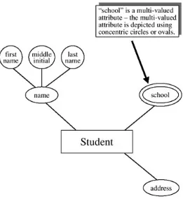
The Multi-Valued Attribute
Another type of non-simple attribute that has to be managed is called a
multi-valued attribute. The multi-valued attribute, as the name implies, may take on more than one value for a given occurrence of an entity. For
Figure 2.5: An ER Diagram with a Multi-Valued
Attribute
Once again, the test of singleversus multi-valued will depend entirely on the circumstances that the database designer encounters — the desire of the "user" for which the database is being built. It is recommended that if the sense of the database is that the attribute school means "current school," then the attribute should be called "current school" and illustrated as a single-valued attribute. In our example, we have a multi-val