High-performance concrete compressive strength prediction using Genetic Weighted Pyramid Operation Tree (GWPOT)

(1)

High-performance concrete compressive strength prediction using

Genetic Weighted Pyramid Operation Tree (GWPOT)

Min-Yuan Cheng, Pratama Mahardika Firdausi

1

, Doddy Prayogo

n,1

Department of Civil and Construction Engineering, National Taiwan University of Science and Technology, #43, Section 4, Keelung Rd., Taipei 106, Taiwan, ROC

a r t i c l e

i n f o

Article history: Received 11 July 2013 Received in revised form 2 October 2013

Accepted 24 November 2013 Available online 15 December 2013

Keywords: Prediction Concrete strength Genetic Algorithm Operation Tree

Weighted Pyramid Operation Tree

a b s t r a c t

This study uses the Genetic Weighted Pyramid Operation Tree (GWPOT) to build a model to solve the problem of predicting high-performance concrete compressive strength. GWPOT is a new improvement of the genetic operation tree that consists of the Genetic Algorithm, Weighted Operation Structure, and Pyramid Operation Tree. The developed model obtained better results in benchmark tests against several widely used artiﬁcial intelligence (AI) models, including the Artiﬁcial Neural Network (ANN), Support Vector Machine (SVM), and Evolutionary Support Vector Machine Inference Model (ESIM). Further, unlike competitor models that use “black-box” techniques, the proposed GWPOT model generates explicit formulas, which provide important advantages in practical application.

1. Introduction

High-performance concrete (HPC) is a new type of concrete used in the construction industry (Yeh, 1998). HPC works better in terms of performance characteristics and uniformity characteris-tics than high-strength concrete (Mousavi et al., 2012; Yeh and Lien, 2009). Apart from the 4 conventional cement ingredients, Portland Cement (PC), water, fine aggregates, and coarse aggre-gates, HPC further incorporates cementitious materials, fly ash, blast furnace slag, and a chemical admixture (Yeh, 1998). These additional ingredients make HPC mix proportion calculations and HPC behavior modeling significantly more complicated than corresponding processes for conventional cement.

Machine learning and AI are attracting increasing attention in academic and empirical ﬁelds for their potential application to civil engineering problems (Mousavi et al., 2012). In civil engineer-ing, AI techniques have been categorized into two approaches, optimization and prediction, with numerous prediction applica-tions including Artiﬁcial Neural Network (ANN), Support Vector Machine (SVM), and Linear Regression Analysis, among others. Optimization applications include the Genetic Algorithm (GA) and Particle Swarm Optimization (PSO).

In the_ﬁeld of civil engineering, much research has focused on hybridizing optimization techniques and prediction techniques. Many papers have reported on hybrid techniques that are able to

predict HPC to a high degree of accuracy (Cheng et al., 2012;Peng et al., 2009;Yeh, 1999). The Evolutionary Support Vector Machine Inference Model (ESIM), one hybridization technique, uses a fast messy Genetic Algorithm (fmGA) and SVM to search simulta-neously for the_ﬁttest SVM parameters within an optimized legal model (Cheng and Wu, 2009). However, the aforementioned techniques, especially ANN, SVM, and ESIM, are considered “black-box” models due to massive node sizes and internal connections. Because these models do not provide explicit for-mulae, they do not explain the substance of the associated model, which is a serious disadvantage in practical applications.

Yeh and Lien (2009) proposed the novel Genetic Operation Tree (GOT) to overcome this disadvantage. The GOT consists of a GA and an Operation Tree (OT). This model is a practical method for eliciting both an explicit formula and an accurate model from experimental data. Although many studies have used GOT to develop formulae to optimallyﬁt experimental data (Chen et al., 2012; Peng et al., 2009; Yeh et al., 2010), this model has yet to achieve results comparable to other prediction techniques such as ANN and SVM. This suggests the potential to further improve the GOT.

This paper introduces a novel approach based on OT called Genetic Weighted Pyramid Operation Tree (GWPOT) to predict HPC compressive strength. The GWPOT integrates the Weighted Operation Structure (WOS) and Pyramid Operation Tree (POT) models to enhance the prediction capability and the ﬁt with experimental data.

Remaining sections in this paper are organized as follows:

Section 2provides a brief explanation of OT, GA, and WOS;Section 3describes the GWPOT model;Section 4describes the case study Contents lists available atScienceDirect

journal homepage:www.elsevier.com/locate/engappai

Engineering Applications of Arti

ﬁ

cial Intelligence

n

Corresponding author. Tel.:þ886 2 27336596; fax:þ886 2 27301074. E-mail addresses:myc@mail.ntust.edu.tw (M.-Y. Cheng),

(2)

and con_ﬁguration of GWPOT parameters, presents GWPOT model results, and compares those results with those of common prediction techniques; and, ﬁnally, Section 5 presents study conclusions.

2. Literature review

2.1. Operation Tree (OT)

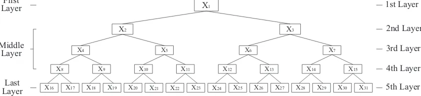
Operation Tree (OT) is a hierarchical tree structure that repre-sents the architecture of a mathematical formula.Fig. 1illustrates an OT model with 31 nodes. InFig. 1, the OT model consists of a root value and sub-trees of children, represented as a set of connected nodes. Each node on the OT model has either 0 or 2 child branches, with the former designated as“leaf nodes”and associated with either a variable or constant and the latter associated with a mathematical formula (þ, , ,C, log, etc.)

(Hsie et al., 2012).Fig. 2shows an example of the OT model with a 31-bit-node code. Table 1 lists the bit codes for mathematical operations, variables, and constants. The OT in Fig. 2 may be expressed as

Output¼ logE

CþD

logEA

AþBþC

D

ð1Þ

Its_ﬂexibility in expressing mathematical formulae allows OT to avoid a disadvantage common to other prediction techniques (Peng et al., 2009; Yeh and Lien, 2009). The branch-and-leaf con_ﬁguration of OT facilitates the deduction of function values and formulae. Input values may thus be substituted into the formula to generate a predicted output value for each data point. OT performance may be evaluated by calculating the root-mean-squared error (RMSE) between predicted and actual output values (Yeh et al., 2010). The best OT formula is achieved when RMSE

reaches the lowest possible value. Because searching the best combination formula toﬁt with the data is a discrete optimization problem, an optimization technique capable of solving a discrete problem must be integrated into the OT model (Peng et al., 2009). 2.2. Genetic Algorithm (GA)

Genetic Algorithm (GA) is an optimization technique _ﬁrst proposed by Holland (1975). GA is based on Darwin's theory of evolution and mimics biological competition in which only com-paratively strong chromosomes survive into the next generation. Each chromosome in a GA population represents a candidate solution for a given problem and is able to generate a result based on the objective function. Ability to handle various types of objective functions is another advantage of GA.

GA proceeds through progressive generations from an initial population. Each GA generation is subjected to genetic operation processes such as evaluation, selection, crossover, and mutation and generates a new result. A new-generation chromosome will replace the current-generation chromosome if it generates a better result.

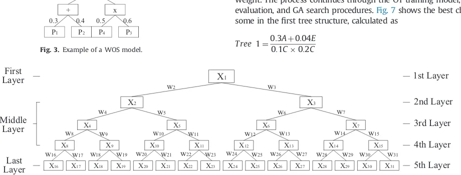
2.3. Weighted operation structure (WOS)

The weighted operation structure (WOS) is an improvement of the OT model proposed byTsai (2011). This study added a constant value to every variable to balance every input variable to help OT generate a better formula. Therefore, WOS assigns weights to every node connection in the OT model so that each WOS element

X9

X4

X2

X

1

X10 X11 X12 X13 X14 X15

X5 X6 X7

X3

X8

X16 X17 X18 X19 X20 X21 X22 X23 X24 X25 X26 X27 X28 X29 X30 X31

First

Layer

Middle

Layer

Last

Layer

1st Layer

2nd Layer

3rd Layer

4th Layer

5th Layer

Fig. 1. Five-layer OT model.

Bits 1 2 3 4 5 6 7 8 9 10 11 12 13 14 15

Code 1 5 2 10 2 3 9 2 5 3 5 7 3 7 4

Bits 16 17 18 19 20 21 22 23 24 25 26 27 28 29 30 31

Code 6 10 9 8 8 9 6 10 7 7 8 6 6 7 8 9

E log

x

+ log B +

/ +

C D A E C A

D /

Fig. 2.Example of an OT model.

Table 1

Genetic code of mathematical operations, variables, and constants.

Code 1 2 3 4 5 6 7 8 9 10

(3)

produces node outputs conducted by 2 OT nodes and 2 undeter-mined weights.

The WOS is thus able to search for the best formula in a wider search space with more combinations over a longer time period than the original OT model. Fig. 3 shows a 5-layer weighted operation structure. The example of the WOS model in Fig. 4

may be expressed as

Output¼ 0:1 ð0:3P1þ0:4P2Þ

0:2 ð0:5P40:6P3Þ¼

0:03P1þ0:04P2

0:012P4P3 ð2Þ 3. Genetic Weighted Pyramid Operation Tree (GWPOT)

3.1. GWPOT architecture

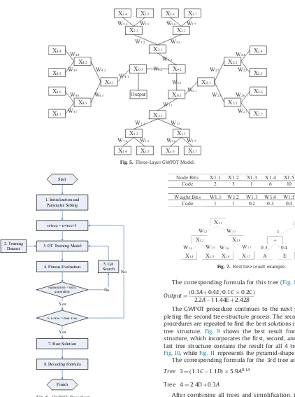
This study proposes a new operation tree algorithm to address the shortcomings of OT called the Genetic Weighted Pyramid Operation Tree (GWPOT). GWPOT applied a pyramid-shaped, 4 connected OT called Pyramid Operation Tree (POT). The signiﬁcantly wider search area of GWPOT results from its use of multiple trees that allows coverage of a greater number of combination possibilities. The weighted concept of WOS was integrated into GWPOT due to the success of this concept in improving GOT performance.Fig. 5 illus-trates a GWPOT model with 3 layers per tree.

Tuning parameters in the GWPOT model include: mutation rate, crossover rate, weight rate, layers per tree, and total number of trees. Mutation rates and crossover rates were retained from OT. The other parameters are new to GWPOT and explained as follows: (1) weight rate sets the probability of each node having a constant value in the WOS structure; (2) layers per tree sets the number of layers used for each tree; and (3) total number of trees sets the number of trees used to produce the formula in one model process. Four trees were used to assemble the pyramid shape in this study. GWPOT operations start by generating a population of chromo-somes for theﬁrst tree. Every chromosome represents the solution vector of formula components. Next, the evaluation step obtains the objective function (RMSE) for each chromosome. Afterward, the GA optimizer searches for the optimal parameter or best formula combination. GA optimization repeats until the stopping criterion is achieved.Fig. 6shows theﬂowchart for GWPOT.

An explanation of the principal steps in GWPOT follows below:

(1) Initialization and parameters setting: This step sets GWPOT tuning

parameters and randomly generates the initial population.

(2) Training dataset: The dataset is divided into two parts, with the

ﬁrst used as training data and the second as testing data.

(3) OT training model: OT is a learning tool able to build an explicit

formula for use as a prediction model. Each chromosome in OT represents one formula, as explained in the previous section of this paper.

(4) Fitness evaluation: A ﬁtness function formula, RMSE in the

current study, evaluates each chromosome. Smaller RMSE values indicate better chromosomes.

(5) GA procedure: GA begins with the selection process. This study

uses a roulette wheel as the selection technique and uniform crossover as the crossover mechanism. After completing cross-over, mutation is performed by generating random real value numbers based on the mutation rate. The termination criterion in the current study is the total number of generations. This GA procedure will repeat until either the stopping criterion or termination criterion is satisﬁed.

(6) Checking the number of tree: If the number of trees does not

reach the maximum parameter value, the GWPOT process continues to the next tree structure. In each new tree struc-ture, the top-half population is generated randomly and includes the best chromosomes from the previous tree struc-ture. Moreover, the amount of bits in every chromosome is expanded in order to modify the current population. The newly added bits are provided to store the formula combina-tion of the next tree structure. The top-half chromosomes from the previous tree are retained due to the possibility that the previous tree structure may not require further change to improve performance. Random numbers replace the bottom-half population in order toﬁnd new tree structure combina-tions. The process continues until the 4th tree is produced.

(7) Optimal solution: The chromosome with the lowest RMSE is

considered to be the optimal solution. This solution is the formula that will be employed to map the input–output relationship of the target dataset.

3.2. GWPOT example

To further clarify the GWPOT procedure, this study applied GWPOT to an example problem. A 3-layer GWPOT was created. This example uses 5 types of operators and variables, respectively. The operators are

,C,þ,–, and \widehat and the variables are A, B, C, D and E. The

weights are set between 0.01 and 10.00, and 4 tree-structure phases must be passed to establish the GWPOT model.

The first tree-structure phase begins by generating a population that is identified by node (variables and mathematical operations) and weight. The process continues through the OT training model,fitness evaluation, and GA search procedures.Fig. 7shows the best chromo-some in thefirst tree structure, calculated as

Tree1¼0:3Aþ0:04E

0:1C0:2C ð3Þ

0.1

+ /

x

P1 P2 P4 P3

0.3 0.4 0.2

0.6 0.5

Fig. 3.Example of a WOS model.

X11 X12 X13 X14 X15

X5 X6 X7

X3

X8

X16 X17 X18 X19 X20 X21 X22 X23 X24 X25 X26 X27 X28 X29 X30 X31

First

Layer

Middle

Layer

Last

Layer

1st Layer

2nd Layer

3rd Layer

4th Layer

5th Layer

w2 w3

w4 w5

w8 w9 w10 w11

w16 w17 w18 w19 w20 w21 w22 w23

w7 w6

w15 w14

w13 w12

w31 w30 w29 w28 w27 w26 w25 w24

X9 X4

X2

X1

X10

(4)

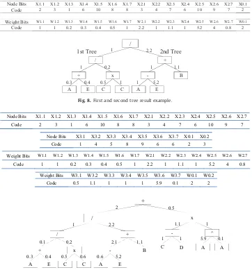
The second tree structure starts with a top-half population generated randomly from the best solutions from thefirst tree structure and augmented by additional new bits. The bottom-half population is tasked to identify new tree structure combinations between thefirst tree and second tree. One additional mathema-tical operator is used to connect the_first tree and second tree. GA finds this operator concurrently using other nodes in the second tree-structure phase. Assuming the first tree solution in the second phase is the same as thefirst tree solution infirst tree-structure phase, the best solution from second tree tree-structure phase may be illustrated as inFig. 8.

The corresponding formula for this tree (Fig. 8) is

Output¼ð0:3Aþ0:4E=0:1C0:2CÞ

2:2A 11:44Eþ2:42B ð4Þ

The GWPOT procedure continues to the next phase after com-pleting the second tree-structure process. The second tree-structure procedures are repeated to_ﬁnd the best solutions in the 3rd and 4th tree structure. Fig. 9 shows the best result from the third tree structure, which incorporates theﬁrst, second, and third trees. The last tree structure contains the result for all 4 trees, as shown in

Fig. 10, whileFig. 11represents the pyramid-shape model.

The corresponding formula for the 3rd tree and 4th trees are:

Tree 3¼ ð1:1C 1:1DÞ 5:9A0:1A ð5Þ

Tree 4¼2:4Dþ0:3A ð6Þ

After combining all trees and simpliﬁcation, theﬁnal formula may be expressed as

Output¼αþβ 2 2 Tree 1

2:2Tree 2þ0:5Tree 3

þ0:5Tree4

ð7Þ

3.3. Modiﬁed predicted output value

An oblique phenomenon frequently occurs in OT-generated for-mula. This phenomenon reﬂects the concurrently high linear correla-tion and high RMSE in the relacorrela-tionship between actual output and predicted output (Yeh and Lien, 2009). To address this problem, some researchers have used single linear regression analysis to modify the OT result (Hsie et al., 2012;Mousavi et al., 2012;Yeh et al., 2010;

X1.2

X1.3

X1.1

X1.4

X1.5

X1.6

X1.7

W1.2

W1.4 W1.5

W1.3

W1.7 W1.6

X

0.1

X0.2

X

2.2

X

2.1

X

2.3

X

2.4

X

2.5

X

2.6

X

2.7 W2.2

W2.4

W2.5

W2.3

W2.7 W2.6

X3.2

X3.3

X3.1

X3.4

X3.5

X3.6

X3.7

W3.2

W3.4 W3.5

W3.3 W3.7 W3.6

Output

X0.3

X

4.2

X

4.1

X

4.3

X

4.4

X

4.5

X

4.6

X

4.7

W4.2 W4.4

W4.5

W4.3

W4.7 W4.6

W1.1

W2.1 W0.1 W0.2 W4.1

W3.1

Fig. 5.Three-Layer GWPOT Model.

1. Initialization and Parameter Setting

n-tree = n-tree+1 Start

3. OT Training Model 2. Training

Dataset

4. Fitness Evaluation 5. GA Search

i-generation = max.

generation No

Yes

6. n-tree = max. tree

Yes

No

7. Best Solution

8. Decoding Formula

Finish

Fig. 6. GWPOTﬂowchart.

W1.2

X1.2 X1.1

X1.3

X1.4 X1.5 X1.6 X1.7

W1.4 W1.5 W1.3

W1.7 W1.6

1

+ /

x

A E C C

0.3 0.4

0.2

1 0.5

Node Bits X1.1 X1.2 X1.3 X1.4 X1.5 X1.6 X1.7

Code 2 3 1 6 10 8 8

Weight Bits W1.1 W1.2 W1.3 W1.4 W1.5 W1.6 W1.7

Code 1 1 0.2 0.3 0.4 0.5 1

(5)

Yeh and Lien, 2009). The practical result of this regression analysis is to assign the same value to the prediction output mean value and the actual output mean value. The equation for the single linear regres-sion analysis is

y¼

α

þ

β

f ð8Þ

wherefis the predicted output value of the operation tree;yis the modiﬁed predicted value;

α

and

β

are the regression coefﬁcients.

According to single linear regression analysis

α

¼y

β

Uf ð9Þ

β

¼∑

n

i¼1ðfi fÞðyi yÞ

∑n

i¼1ðfi fÞ2

ð10Þ

whereyis the mean of actual output values in the dataset;fis the mean of predicted output values in the dataset;yiis the actual output value of theith data in the dataset; andfiis the predicted output value of theith data in the dataset.

4. Case study

4.1. The dataset

The dataset used was obtained fromYeh (1998) and published in the data repository of the University of California, Irvine (UCI). A

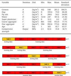
total of 1030 concrete samples covering 9 variables were collected from the database. Eight of the 9 variables or in_fluencing factors in the dataset, including cement, fly ash, slag, water, SP, coarse aggregate,fine aggregate, and age, were treated as input variables. The remaining variable, concrete compressive strength, was trea-ted as the output variable.Table 2shows descriptive statistics for these factors.

4.2. Tuning parameters

In this study, each parameter was set as: crossover rate¼0.8, mutation rate¼0.05, and weighted rate¼0.5. Moreover, the total tree was set at 4, with 3, 4, 5, and 6 layers. Furthermore, the total population size and the total number of generations for each tree selected for this study were 100 and 2,000, respectively.

4.3. k-Fold cross validation

k-Fold cross validation is a statistical technique that divides study data into k subsamples to determine the accuracy of a prediction model. The original data is divided randomly into k equally sized or approximately equally sized segments, with one subsample used as testing data and the remainingk–1 subsamples used as training data. The cross validation process recreates the 1

+ /

x

A E C C

0.3 0.4 0.2

1 0.5

1

-+

B

A E

1 5.2 1.1

/

1 2.2

2nd Tree

1st Tree

Node Bits X1.1 X1.2 X1.3 X1.4 X1.5 X1.6 X1.7 X2.1 X2.2 X2.3 X2.4 X2.5 X2.6 X2.7 X0.1

Code 2 3 1 6 10 8 8 3 4 7 6 10 9 7 2

Weight Bits W1.1 W1.2 W1.3 W1.4 W1.5 W1.6 W1.7 W2.1 W2.2 W2.3 W2.4 W2.5 W2.6 W2.7 W0.1 Code 1 1 0.2 0.3 0.4 0.5 1 2.2 1 1.1 1 5.2 4 0.8 2

Fig. 8.First and second tree result example.

Node Bits X1.1 X1.2 X1.3 X1.4 X1.5 X1.6 X1.7 X2.1 X2.2 X2.3 X2.4 X2.5 X2.6 X2.7

Code 2 3 1 6 10 8 8 3 4 7 6 10 9 7

Node Bits X3.1 X3.2 X3.3 X3.4 X3.5 X3.6 X3.7 X0.1 X0.2

Code 1 4 5 8 9 6 6 2 3

Weight Bits W1.1 W1.2 W1.3 W1.4 W1.5 W1.6 W1.7 W2.1 W2.2 W2.3 W2.4 W2.5 W2.6 W2.7

Code 1 1 0.2 0.3 0.4 0.5 1 2.2 1 1.1 1 5.2 4 0.8

Weight Bits W3.1 W3.2 W3.3 W3.4 W3.5 W3.6 W3.7 W0.1 W0.2

Code 0.5 1.1 1 1 1 5.9 0.1 2 2

C D A A

1.1

1 1

1

0.1 5.9 +

2 0.5

0.1

+ /

x

A E C C

0.3 0.4 0.2

0.6 0.5

2.1

-+

B

A E

0.6 5.2 1.1 /

1 2.2

- ^

x

(6)

modelktimes, with each ksubsample used exactly once as the validation data. Results from all subsamples or from all folds are then averaged to produce a single value estimation.

In general, becausekremains an unﬁxed parameter, the value ofkmay be any suitable number. The current study set the value of kas 5 in order to limit total computational time. Five-fold means that each set uses 20% of the data (206 data points) as testing data and 80% (824 data points) as training data. The data contains 1030 HPC records is divided randomly into 5 equally sized (206 data), with one subsample used as testing data and the remaining 4 subsamples used as training data. Five-fold means that each set uses 20% of the data (206 data points) as testing data and 80% (824 data points) as training data. The cross validation process recreates the model 5 times, with each 5 subsample used exactly once as the validation data.Fig. 12illustratesk-fold cross valida-tion operavalida-tions.

4.4. Performance measurement

To explore the accuracy of each model, this study used 3 performance-measurement equations: Root Mean Square Error Node Bits X1.1 X1.2 X1.3 X1.4 X1.5 X1.6 X1.7 X2.1 X2.2 X2.3 X2.4 X2.5 X2.6 X2.7

Code 2 3 1 6 10 8 8 3 4 7 6 10 9 7

Node Bits X3.1 X3.2 X3.3 X3.4 X3.5 X3.6 X3.7 X4.1 X4.2 X4.3 X4.4 X4.5 X4.6 X4.7

Code 1 4 5 8 9 6 6 3 9 6 6 8 7 7

Code 1 1 0.2 0.3 0.4 0.5 1 2.2 1 1.1 1 5.2 4 0.8

Code 0.5 1.1 1 1 1 5.9 0.1 0.5 2.4 0.3 8 2.7 9.2 0.1

Node Bits X0.1 X0.2 X0.3 Weight Bits W0.1 W0.2 W0.3

Code 2 3 3 Code 2 2 2

C D A A

1.1

1 1

1

0.1 5.9

+

2 0.5

D A

+

2.4 0.3

+

2 0.5

0.1 +

/

x

A E C C

0.3 0.4 0.2

0.6 0.5

2.1

-+

B

A E

0.6 5.2 1.1

/

1 2.2

- ^

x

Fig. 10.Four-tree result example.

+ x

/

A E C C

1

0.3 0.4

0.2

1 0.5

/ +

B

+

-E

A

1.1

1

1 5.2

^

-x

A A D C

1

0.1 5.9

1.1 1 1

Output

+ D

+

A

2.4

0.3

1 2.2 2 2

0.5

Fig. 11. GWPOT result example.

Table 2

HPC variables data.

Variable Notation Unit Min Max Mean Standard deviation

Cement A (kg/m3

) 102 540 281.2 104.51

Slag B (kg/m3

) 0 359.4 73.9 86.28

Fly ash C (kg/m3

) 0 200.1 54.2 64.00

Water D (kg/m3

) 121.8 247 181.6 21.36 Super plasticizer E (kg/m3₎ ₀ _32.2 _6.2 _5.97 Coarse aggregate F (kg/m3

) 801 1145 972.9 77.75 Fine aggregate G (kg/m3

) 594 992.6 773.6 80.18

Age H Day 1 365 45.7 63.17

Compressive atrength

Output MPa 2.3 82.6 35.8 16.71

set 1

set 2

set 3

set 4

set 5

fold 5

fold 1 fold 2 fold 3

fold 1 fold 2 fold 3 fold 4

fold 4

fold 5

training data

training data testing data

training data training data testing data

training data testing data training data training data testing data

(7)

(RMSE), Mean Absolute Error (MAE), and Mean Absolute Percen-tage Error (MAPE). All performance measures used in testing data were combined to create a normalized reference index (RI) in order to obtain an overall comparison (Chou et al., 2011). Each ﬁtness function was normalized to a value of 1 for the best performance and 0 for the worst. The RI was obtained by calculating the average of every normalized performance measure as shown in Eq.(11). Eq.(12)shows the function used to normalize the data.

RI¼RMSEþMAEþMAPE

3 ð11Þ

xnorm¼ ðxmax xiÞ

ðxmax xminÞ ð12Þ

4.4.1. Root mean square error

Root mean square error (RMSE) is the square root of the average squared distance between the model-predicted values and the observed values. RMSE may be used to calculate the variation of errors in a prediction model and is very useful when large errors are undesirable. RMSE is given by the following equation:

RMSE¼

ffiffiffiffiffiffiffiffiffiffiffiffiffiffiffiffiffiffiffiffiffiffiffiffiffiffiffiffiffiffiffiffiffi

1

n∑

n

j¼1ðyj y^jÞ2

r

ð13Þ

whereyjis the actual value;yjis the predicted value; andnis the number of data samples.

4.4.2. Mean absolute error

Mean absolute error (MAE) is the average absolute value of the residual (error). MAE is a quantity used to measure how close a prediction is to the outcome. The MAE may be expressed as

MAE¼1

n∑

n

j¼1jyj y^jj ð14Þ

whereyjis the actual value;y^jis the predicted value; andnis the number of data samples.

4.4.3. Mean absolute percentage error

Mean absolute percentage error (MAPE) calculates percentage error of prediction. Small denominators are problematic for MAPE because they generate high MAPE values that impact overall value. The MAPE may be expressed as

MAPE¼1

n∑

n j¼1

yj y^j

yj

100% ð15Þ

whereyjis actual value;y^jis predicted value; andnis number of data samples.

4.5. Results and discussion

This study compared the performance of the proposed model against two other OT-based tools, the Genetic Operation Tree (GOT) and the Weighted Operation Structure (WOS). After testing a variety of layer numbers, the number of layers needed to build the best GWPOT model formula was determined as between 3 and 6.

Five-fold cross-validation techniques validated the perfor-mance of the models. The average 5-fold results for GOT, WOS, and GWPOT are summarized inTables 3–5, respectively.

Table 3shows that the 5-layer conﬁguration generated the best RI result for the GOT model (0.817). Eq.(16)shows the formula associated with this result. On the other hand, the six-layer conﬁguration generated the best overall and average for the WOS model (0.872). Eq.(17) shows the formula associated with this result.

y¼2:905þ0:077 logðAHþH

2

Þ logðlnðDþHÞÞ

!ðlogðAþBþlnCÞ=logDÞ 0

@

1

A ð16Þ

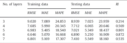
The RI results in Table 5 for the 3-, 4-, 5-, and 6-layer configurations are: 0.263, 0.448, 0.695, and 0.690, respectively. This indicates that the 5-layer configuration generated the best RI result for the GWPOT model. The 6-layer configuration generated the worst result due to increased model complexity and large chromosome bit number. Further, larger layer numbers require more computational time, which increases the difficulty offinding the best combination.

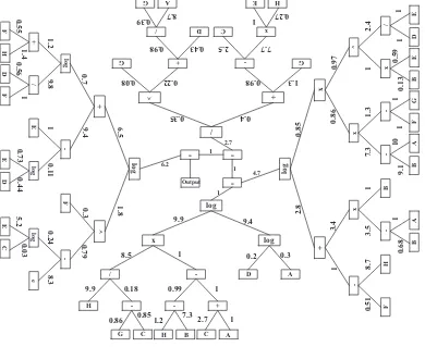
Fig. 13illustrates the best OT produced using GWPOT. The OT in

Fig. 13is generated from the best 5-layer GWPOT model and may Table 3

Average of GOT performance measurements results.

No. of layers Training data Testing data RI RMSE MAE MAPE RMSE MAE MAPE 3 10.226 8.250 30.735 10.415 8.400 31.282 0.136 4 8.105 6.394 22.741 8.066 6.429 23.092 0.600 5 7.117 5.537 18.661 7.120 5.509 18.611 0.817 6 7.005 5.465 18.573 7.357 5.681 19.049 0.779 7 7.270 5.637 19.425 7.253 5.615 19.033 0.792

Table 4

Average of WOS performance measurement results.

No. of layers Training data Testing data RI RMSE MAE MAPE RMSE MAE MAPE 3 9.020 7.089 24.853 8.939 7.025 23.959 0.214 4 7.685 5.990 20.345 7.712 6.065 20.646 0.569 5 6.983 5.405 18.540 7.021 5.349 18.437 0.801 6 6.646 5.070 16.668 6.890 5.230 16.909 0.872 7 6.801 5.169 17.307 7.410 5.549 18.160 0.535

Table 5

Performance measurement results of GWPOT model.

No. of layers Training Testing RI

RMSE MAE MAPE RMSE MAE MAPE 3 6.825 5.273 17.490 7.050 5.442 18.333 0.263 4 6.352 4.877 16.335 6.780 5.174 17.253 0.448 5 5.864 4.440 14.986 6.379 4.787 16.095 0.695 6 5.689 4.307 14.597 6.446 4.750 16.118 0.690

y¼ 35:74þ2:842 log 9:9H

ðlog ðð3:173Aþ3:188Bþ1:033C 2:922DÞ ð2:467Eþ0:262H 0:725A 0:125FÞÞ=logð2:798D ln ln 83:025EÞÞ

(8)

be decoded into a complete formula using Eqs. (18) through(22).

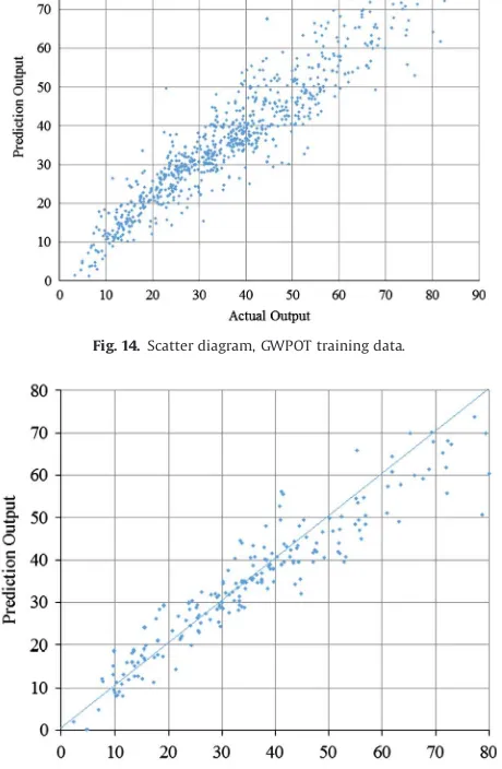
Figs. 14and15 show scatter diagrams for the actual values and predicted values of, respectively, training data and testing data.

x1¼First tree output

¼lnðð833:085H=13:026G 12:875CÞ ð11:761H 71:547B 26:73C 9:9AÞÞ ln log1:88A2:82D

ð18Þ

x2¼Second tree output¼

lnð1:428F 2:436Hþ215:704B2 ₃₁₇ :206ABÞ lnðð48:56B 53:363AÞð0:95F 0:95GÞðð0:052BEÞD=E_ÞÞ

ð19Þ

x3¼Third tree output¼

0:52Gþ2:46EH 0:98C

ð0:033Dþ ð0:657A=0:029GÞÞ0:028G ð20Þ

y¼ 90:089þ17:628ðx1 4:7x2 2:7x3 6:2x4Þ ð22Þ

Wider search area allows GWPOT to precisely identify the relationships between all the input variables (variablesAthrough H) and the prediction output. Meanwhile, the result shows that GOT and WOS exclude some input variables. In the GOT formula example (Eq. (16)), super plasticizer, ﬁne aggregate, and coarse aggregate are not included in the formula. Peng et al. stated that excluding some variables from a formula does not mean they do not impact the compressive strength (Peng et al., 2009). The GWPOT depicts the relationship between all input–output

variables and shows that each variable has a distinct inﬂuence on HPC compressive strength.

This study compared 3 types of OT to verify that the proposed new OT outperforms the other two. The best-solution conﬁ gura-tion for each OT was determined and used in this comparison. These conﬁgurations were: 5-layer for the GOT model, 6-layer for the WOS model, and 5-layer for the GWPOT model. Table 6

summarizes comparisons among these models.

GWPOT obtained the best result for every performance mea-sure, with an RI value of 1.00. GOT and WOS obtainedRIvalues of 0.00 and 0.458, respectively. Due to the superior performance of GWPOT over the two other OT models, the GWPOT model was tested against other prediction techniques.

4.6. Comparison

This section presents the results of comparing GWPOT to other prediction techniques including SVM, ANN, and ESIM. The GWPOT result was obtained as explained in the previous section using a 5-layer model in fold set one, and 5-fold cross validation was performed on all results. Table 7 presents model results for comparison.

GWPOT obtained a better RI value than SVM and ANN but worse than ESIM. ESIM demonstrated its superiority with a prediction RI value of 0.918 compared to RI values for GWPOT, SVM, and ANN of 0.085, 0.072, and 0.684, respectively. Although

F ^ log e -E C 0.24 8.3 5.2 0.03 / log + E log -+ FH D F 1.2 9 .8 1 0.11 0.56 0.73 0.44 0.55 1.4 1 ED log 0.7 9.4 6.5 0.79 0.3 1. 8 -Output -1 4.7 1 1 6.2 2.7 D log A -/ x - + -H

G C H B

9.9 0.18 0.99 1

0.86 0.851.2 7.3 2.7 1

C A log 8.5 1 9.9 0.3 0.2 9.4 -x x x / ^ -BA F G BE 7.3 1.3 1 2.4 1 1 1 9.1 10 0.13 0.59 1 DE H -+ -B x F BA 0.51 8.7 3.5 1 0.68 1 log 1 3.4 2.8 0.97 0.86 0.85 / + ^ G D A G 0.43 0.98 8.7 0.39 G + x C -HE 7.7 2.5 0.27 1 / 1.3 0.98 0.4 0.08 0.22 0.35

Fig. 13. Best solution GWPOT model.

x4¼Fourth tree output¼

lnððlog_ð24:97D=44:59FÞð3:003Fþ7:644HÞÞ þ6:11E log2:957D4:906EÞ

(9)

theRIvalue for GWPOT fell short of theRIvalue for ESIM, GWPOT remains capable of competing with ESIM, as demonstrated by the superior RMSE value obtained by GWPOT (6.379) compared to ESIM (6.574).

4.7. Sensitivity analysis

OT uses a single-tree structure to build its model while GWPOT uses 4 trees to form a pyramid shape. Other OT model conﬁ gura-tions such as 2-tree and 3-tree exist as well. To increase the validity of the GWPOT concept, this study conducted another comparative analysis that used various combinations of layer numbers and tree numbers to identify differences among these parameters. Each tree number and layer number used the 5-fold

cross validation technique to avoid potential bias.Table 8shows averageRIresults for each fold set.

As shown in Table 8, the 5-tree structure with 4 layers generated the best result with anRIvalue of 0.792. The 5-tree, 5-layer model obtained a good result of 0.790, which differed only slightly from the bestRIsolution. The worstRIresult was 0.296, produced by the 1-tree, 3-layer model.

The unexpected results and the _ﬂexibility of the solution indicate that another OT model may generate the ultimate best solution. However, the 4-tree, 5-layer model obtained the best result in this study.

5. Conclusions

This study develops a new GWPOT to predict HPC compressive strength. Accurately predicting HPC strength is critical to building a robust prediction model for HPC. The GWPOT model employs 4 hierarchical OT to form the pyramidal shape. Multiple trees widen the GA search area, creating a formula that is more complex and moreﬂexible toﬁt with the data. Comparisons between GWPOT and other prediction techniques, including GOT, WOS, SVM, ANN, and ESIM, showed the highly competitive performance of GWPOT in predicting HPC compressive strength.

GWPOT performs comparably to the well-known ESIM in terms of prediction accuracy. However, while ESIM uses a black-box approach that does not depict input–output relationships in an explicit formula, GWPOT generates and shows corresponding formulae for these relationships. This comparative transparency gives GWPOT an important advantage in practical applications. In future research, another optimization technique may be devel-oped to replace the GA technique used in this study for further comparison. Additionally, the efﬁcacy of GWPOT may be further tested and veriﬁed on other construction management case studies.

References

Chen, K.-T., Kou, C.-H., Chen, L., Ma, S.-W., 2012. Application of genetic algorithm combining operation tree (GAOT) to stream-way transition. In: Proceedings of the 2012 International Conference on Machine Learning and Cybernetics, vol. 5. IEEE, Xian, China, pp. 1774–1778.

Table 6

Performance measurement results of various OT techniques.

Prediction tools Training Testing RI

RMSE MAE MAPE RMSE MAE MAPE GOT 7.117 5.537 18.661 7.120 5.509 18.611 0.000 WOS 6.646 5.070 16.668 6.890 5.230 16.909 0.458 GWPOT 5.864 4.440 14.986 6.379 4.787 16.095 1.000

Table 7

Performance measurement results of various prediction techniques.

Prediction technique Training Testing RI RMSE MAE MAPE RMSE MAE MAPE SVM 6.533 4.610 16.356 7.170 5.295 18.610 0.085 ANN 6.706 5.189 18.761 6.999 5.416 19.632 0.072 ESIM 3.294 1.597 5.191 6.574 4.160 13.220 0.918 GWPOT 5.864 4.440 14.986 6.379 4.787 16.095 0.684

Table 8

RIValues from various layer and tree number conﬁgurations. Number of trees Number of layers

3 4 5 6

1 0.2960 0.5341 0.6665 0.7283

2 0.5820 0.6766 0.7241 0.7752

3 0.6569 0.7128 0.7654 0.7858

4 0.6764 0.7354 0.7901 0.7693

5 0.7197 0.7419 0.7823 0.7537

Fig. 14.Scatter diagram, GWPOT training data.

(10)

Cheng, M.-Y., Chou, J.-S., Roy, A.F.V., Wu, Y.-W., 2012. High-performance concrete compressive strength prediction using time-weighted evolutionary fuzzy sup-port vector machines inference model. Automat. Constr. 28, 106–115. Cheng, M.-Y., Wu, Y.-W., 2009. Evolutionary support vector machine inference

system for construction management. Automat. Constr. 18, 597–604. Chou, J.-S., Chiu, C.-K., Farfoura, M., Al-Taharwa, I., 2011. Optimizing the prediction

accuracy of concrete compressive strength based on a comparison of data-mining techniques. J. Comput. Civ. Eng. 25, 242–253.

Holland, J.H., 1975. Adaptation in Natural and Artiﬁcial Systems. University of Michigan Press.

Hsie, M., Ho, Y.-F., Lin, C.-T., Yeh, I.C., 2012. Modeling asphalt pavement overlay transverse cracks using the genetic operation tree and Levenberg–Marquardt Method. Expert Syst. Appl. 39, 4874–4881.

Mousavi, S.M., Aminian, P., Gandomi, A.H., Alavi, A.H., Bolandi, H., 2012. A new predictive model for compressive strength of HPC using gene expression programming. Adv. Eng. Software 45, 105–114.

Peng, C.-H., Yeh, I.-C., Lien, L.-C., 2009. Building strength models for high-performance concrete at different ages using genetic operation trees, nonlinear regression, and neural networks. Eng. Comput. 26, 61–73.

Tsai, H.-C., 2011. Weighted operation structures to program strengths of concrete-typed specimens using genetic algorithm. Expert Syst. Appl. 38, 161–168. Yeh, I.-C., 1998. Modeling of strength of high-performance concrete using artiﬁcial

neural networks. Cem. Concr. Res. 28, 1797–1808.

Yeh, I.-C., 1999. Design of high-performance concrete mixture using neural net-works and nonlinear programming. J. Comput. Civ. Eng. 13, 36–42.

Yeh, I.-C., Lien, C.-H., Peng, C.-H., Lien, L.-C., 2010. Modeling concrete strength using genetic operation trees. In: Proceedings of the 2010 International Conference on Machine Learning and Cybernetics, vol. 3. IEEE, Qindao, China, pp. 1572– 1576.