A generalized environmental sustainability
index for agricultural systems
Gary R. Sands
a,∗, Terence H. Podmore
a,baDepartment of Biosystems and Agricultural Engineering, University of Minnesota, 1390 Eckles Ave., St Paul, MN 55108, USA bDepartment of Chemical and Bioresource Engineering, Colorado State University, Fort Collins, CO 80521, USA
Received 30 July 1997; received in revised form 11 May 1999; accepted 21 October 1999
Abstract
This paper presents the design and development of an Environmental Sustainability Index (ESI) and describes a case study used to evaluate the performance of the index. The objective of the index was to provide a modelling-based, quantitative measure of sustainability from an environmental perspective, comprising both on- and off-site environmental effects associated with agricultural systems. A performance approach was utilized for the ESI, having inputs that were derived from long-term simulations of crop management systems with the EPIC model (Erosion Productivity Impact Calculator). 15 sub-indices for representing sustainability were chosen employing a dual framework for characterizing environmental sustainability, embodying the agricultural system’s: (i) inherent soil productivity and groundwater availability; and (ii) potential to degrade the surrounding environment. A case study was developed based on prevalent corn and wheat agricultural production systems in Baca County, located in southeastern Colorado. Principal components analysis was employed to assess the information content of the 15 sustainability sub-indices. Sensitivity analysis was performed to evaluate the effects of model input uncertainty on the index. The effect of the time frame over which the index is computed was also examined for time frames ranging from 50 to 300 years. Results show that the ESI is capable of demonstrating clear differences among crop management systems with respect to sustainability. © 2000 Elsevier Science B.V. All rights reserved.
Keywords: Sustainable agriculture; Environmental impacts; Agricultural systems; Index number theory
1. Introduction
Of all human activities, it is perhaps agriculture that alters the global environment to the greatest ex-tent (CAST, 1994). The paradigm for agricultural development in the US has taken some remarkable turns over the past two centuries. Still dogged by the threat of soil degradation, modern, industrialized
agri-∗Corresponding author. Tel.:+1-612-625-4756; fax:+1-612-625-3005.
E-mail address: [email protected] (G.R. Sands)
culture is especially hard on the environment (Stein, 1992). Water depletion and degradation, threats to human health, genetic diversity, and habitat alteration are all part of the litany of environmental ills asso-ciated with modern agriculture. The current struggle, pitting ‘conventional’ and ‘alternative’ agriculture paradigms, in both research and practice, comes in the wake of unparalleled, yet bittersweet harvests of the Green Revolution era. Today, agriculture’s scien-tific and production communities face the challenge of developing a new paradigm for agriculture which embodies the concept of sustainability. No longer is
production for production’s sake an acceptable goal. Sustainability for agriculture implies food and fiber production with a mission: production which guar-antees ecological stability, economic viability and socio-cultural permanence (Lal, 1991).
Although sustainability has become one of the forefront issues faced by agriculture, ‘sustainable agriculture’ continues to remain an ill-defined con-cept. Despite broad use of the term, the current literature still wrestles with developing and refining the concept. There appears to be some consensus among researchers on perhaps the most general def-inition of sustainability, ‘meeting the needs of the present without compromising the ability of future generations to meet their own needs’ (WCED, 1987). Pragmatic definitions of sustainability however, have been evolving at a much slower pace over the past decade.
This research was motivated by the premise that the concept of sustainability must move from a qualitative state to a quantitative form, in order for sustainability to serve as a guide for agricultural development ini-tiatives. Indeed, many researchers feel that the pres-ence of conceptual inconsistencies and the abspres-ence of operational definitions have hampered attempts to appraise, let alone achieve, sustainability (Brklacich et al., 1991; Lal, 1991; Senanayake, 1991). Hailu and Runge-Metzger (1992) agree that ‘surprisingly little thought has been devoted, however, to devis-ing a sound methodology for recognizdevis-ing when land management practices actually are sustainable and when they aren’t.’ According to Senanayake (1991), developing a quantitative measure of sustainability is an important prerequisite to the development of legislative measures for agriculture, such as those be-ing enacted in many countries today. On appraisbe-ing sustainability, Lal (1991) mandated that the primary concern is not whether sustainability is important or not, but ‘. . .how to use the concept of sustainability in practical and operational terms to alleviate the press-ing problems and production constraints of modern agriculture.’
Hansen (1996) thoroughly reviewed approaches to the concept of sustainability by examining barriers to use of the concept as a criterion for guiding change. He identified two broad interpretations of the concept of sustainability: an approach to agriculture and a property of agriculture. He proposed that as a useful
criterion for change in agriculture, sustainability should be characterized with literal, system-oriented, quantitative, predictive, stochastic and diagnostic properties. Others have proposed theoretical frame-works for evaluating sustainability, using various scales and disciplinary emphasis (Liverman et al., 1988; Lal, 1991; Senanayake, 1991; Stockle et al., 1994). A common emergent theme is that sustain-ability embodies environmental, economic, and social dimensions (Douglass, 1984). Ideally, a holistic ap-praisal of sustainability should integrate these three dimensions (Allen et al., 1991). Although perhaps an ideal approach, integrating three dimensions of sustainability would be extremely difficult in a first attempt at quantifying the concept, owing to the complexity of each dimension. Therefore, a more pragmatic approach toward quantifying sustainabil-ity would be to start with these three dimensions on an individual basis and work towards an integrated measure.
2. Methods
The ESI is a performance-based measure of an agricultural system in that it provides a measure of the performance of an agricultural system over time, in contrast to a representation of its state or condition at any one particular time. Computation of the ESI involves two fundamental steps: (1) simulation of crop management system performance over a selected time frame, and (2) computation of the ESI based on simulation model outputs. The Erosion Productivity Impact Calculator (EPIC), version 3090 (Williams et al., 1982) was used for simulating the performance of agricultural systems. ESI computations were per-formed using commercial spreadsheet applications software, on an Intel-based platform. The following sections describe the conceptual and computational aspects of the ESI and its various components.
2.1. Definition of environmental sustainability
The operative definition of environmental sustain-ability is based on a dual framework embodying both on- and off-site environmental effects of an agricul-tural system. Two sustainability axioms were devel-oped, based on this dual framework, and serve as a reference point or datum from which the performance of agricultural systems can be compared.
Axiom 1 (Environmental sustainability). An envi-ronmentally sustainable agricultural system is one in which the inherent capacity of the soil and wa-ter resources that support agricultural production are maintained or improved over time.
An important distinction between productivity and production must be made. The inherent capacity to support production has to do with intrinsic properties of the resources (i.e., their quality and quantity) and not simply maintenance of productivity in the conven-tional sense. In the convenconven-tional sense, maintaining soil productivity is analogous to producing consistent yields by supplying inputs to the system as necessary, provided that they are economically justified. In the sustainability context however, a soil’s productivity can only be maintained if the intrinsic characteristics that make the soil productive in the first place (e.g.,
tilth, organic matter, favorable structure) are main-tained or improved.
An illustration of this concept is the role of soil organic matter, considered by many to be the sin-gle most important determinant of inherent soil pro-ductivity. When soil organic matter is mined through agricultural production, the soil’s inherent productiv-ity declines despite the fact that yields can be main-tained by making various soil amendments. Hence, to be sustainable, an agricultural system must exhibit signs that this inherent productivity is maintained, and not mined, over time.
Axiom 2 (Environmental sustainability). An environ-mentally sustainable agricultural system is one where no leaching, lateral flow, and/or runoff of degradative constituents occurs (i.e., nutrients, agricultural chem-icals, and sediment).
This second criterion of sustainability provides for a connection of the agricultural system with the off-site or downstream environment, so that sustainability at the system or farm level does not exclude or preclude sustainability at the larger scale. With the exception of soil loss through wind erosion, air quality effects have been excluded from consideration in Axiom 2. The operative definition of environmental sustainability is then as follows: An agricultural system is considered to be environmentally sustainable if certain inherent qualities of soil and water resources are maintained and no drift of nutrients, chemicals or sediment occurs from the system. This axiomatic definition thus estab-lishes a convenient reference point for sustainability, from which to measure and compare the performance of agricultural systems.
2.2. Spatial and temporal scales
from EPIC. The most appropriate analytical time frame for sustainability considerations is still con-tentious, thus, evaluation of the analytical time frame was one of the important objectives of this research.
2.3. Structure of the ESI
The resource productivity and off-site pollution components of environmental sustainability were each considered a conceptual sub-unit of the ESI, expressed symbolically as follows:
ESI=f{SIi} i=1 to 15
SIi =f
Ri, Dj i=1 to 10 j =1 to 5
Ri =f{Pi,GW} i=1 to 4
Di=fSi, Lj i=1 to 3 j=1 to 2
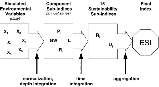
SIi represents a group of 15 sustainability sub-indices. Riis a collection of soil and water resource sub-indices including inherent soil productivity, Pi, and groundwa-ter availability, GW. Di is a collection of sub-indices characterizing the losses from the agricultural system via surface processes, Si, and leaching processes, Li. The sub-indices, Pi, GW, Si, and Liare based on trans-formations of daily model outputs obtained from sim-ulations of the agricultural system. Fig. 1 portrays, from left to right, the ESI’s computational steps from daily outputs, to annual sub-indices, to ‘sustainability sub-indices’ (Ri and Di), which are ultimately aggre-gated to produce the ESI.
Fig. 1. Flow of information and computation of the ESI.
2.4. The resource sustainability sub-indices, Ri
The resource sustainability sub-indices, Ri, charac-terize the status of specific soil and water resources over the simulation period, in response to agricul-tural management practices. A number of resource variables was chosen to represent various characteris-tics of the soil and water resources upon which agri-cultural systems depend for their continued function. These model-simulated resource variables were then transformed in several steps, into annual ‘resource sub-indices’.
2.4.1. The soil property sub-indices, Pi
The soil property sub-indices are a representation of the physical, biological, and chemical changes that occur in the soil from the effects of agricultural pro-duction activities and climatic factors. Four soil prop-erties were chosen: topsoil depth (TS), soil organic carbon (OC), total available water capacity (AW), and bulk density, (BD). Additional properties could have been included, but these four were considered to be sufficient. The formulation of these soil property sub-indices was based on the productivity index of Neill (1979), as modified by Pierce et al. (1983), and the soil tilth index proposed by Singh et al. (1992).
Fig. 2. Bulk density indices for various soil textures (adapted from Pierce et al., 1983).
a non-limiting condition for crop growth and 0 sig-nifies a no-growth condition with regard to the par-ticular soil property. Fig. 2, the bulk density property index, serves as an illustration of the transformation of model-simulated soil characteristics to normalized soil property sub-indices. A depth-weighting process was used for integrating each soil characteristic over the rooting profile, to obtain a single daily index for each characteristic. Further details of the soil property sub-indices are described in Sands (1995).
2.4.2. The groundwater resource sub-index
The groundwater resource sub-index (GW) was de-signed to reflect the effect of agriculture on the US high plains water resource, the Ogallala aquifer, over time. The Ogallala aquifer is the primary source of wa-ter for irrigation in the central US, including Nebraska, Kansas and northern Texas, western Oklahoma, and the eastern regions of Wyoming, Colorado, and New Mexico. In the areas where the Ogallala formation sus-tains irrigated agriculture, rates of recharge are gener-ally small compared with rates of withdrawal (Opie, 1993). Mining of the Ogallala aquifer as a sustaining water resource is the concern in these regions, and hence, forms the basis of GW.
The GW is based on a gross annual aquifer recharge budget, an initial saturated thickness for the aquifer, and the specific yield of the aquifer formation. As with the other resource sub-indices, GW has a value between 0 and 1. GW is initialized to a value of 1 to begin a simulation period. GW then decreases linearly
(if use > recharge) in proportion to the annual budgeted saturated thickness of the aquifer, computed by the following formulae:
RBi =RBi−1+
(Perci−Wi) Sy
, fori=1,nyrs
RB0=b
where RBi is the annual aquifer recharge budget, b is the initial saturated thickness of the aquifer (input variable); Perci is the simulated annual water percola-tion below the root zone; Wi is the simulated annual groundwater withdrawal; Sy, is the aquifer specific yield (meters of water yield/per meter of drawdown); and nyrs is the number of years in the simulation pe-riod. It must be stressed that RB is not derived from a water table simulation; it is merely an indication of aquifer use, based on simulated quantities of percola-tion and water withdrawal.
2.4.3. Time aggregation of the resource sub-indices
The ESI computations thus described produce a se-ries of annual values for each of the five resource sub-indices, TS, BD, AW, OM, and GW, where the number of values is nyrs. Two measures were extracted from each annual series to characterize the agricul-tural system’s effect on the resources (or soil property) over time. Each of the five annual series of sub-index values is thus reduced to two measures, resulting in a total of 10 resource sustainability sub-indices. These 10 resource sustainability sub-indices were previously referred to collectively, as mentioned earlier, as Ri.
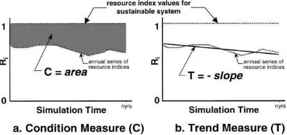
Fig. 3 illustrates the two measures extracted from the five annual resource sub-indices (TS–GW). The ‘condition’ measure, C, characterizes the overall
Fig. 3. The condition, C, and trend, T, aggregation measures, where nyrs is the number of simulation years and Ri is any one
magnitude of the difference of a particular resource sub-index from the ideal state value of 1.0, over the simulation period. C is computed by integrating the area between the sub-index values and the value of 1.0, shown as the shaded region in Fig. 3a. As a decreasing scale measure, smaller values of C indi-cate a more sustainable condition (i.e., the resource sub-indices lie closer to the value of 1.0). Each re-source sub-index, once transformed, is assigned a subscript of C (e.g., TSC, BDC).
The ‘trend’ measure, T, describes the overall lin-ear trend of a resource sub-index over the simulation period. Fig. 3b shows that T is computed as the nega-tive of the slope resulting from a linear regression of the resource sub-index on time. Positive values of T indicate a less sustainable condition (i.e., trend away from the value of 1.0). A negative value of T indicates an improvement in the resource over time. The max-imum and minmax-imum values of T are 1.0 and −1.0, respectively, for the extreme case in which a resource sub-index changes from 0 to 1 or from 1 to 0 within a 1 year period. Each resource sub-index, once trans-formed, is assigned a subscript of T (e.g., TST, BDT).
2.5. The off-site impact sub-indices, Di
Five sub-indices were designed to represent an agricultural system’s potential to degrade the sur-rounding (or downstream) environment because of losses from the system. These sub-indices were de-rived from EPIC’s simulated annual leaching, runoff and airborne mass losses of potentially degradative constituents (i.e., nutrients, sediment, and agricultural chemicals) from the agricultural system. Li and Ri represent two leaching sub-indices (nitrate-nitrogen and pesticides) and three runoff sub-indices (nutri-ents, sediment, and pesticides), respectively. The sed-iment component of Ri also includes sediment loss via wind erosion. These sub-indices were designed to embody elements of both frequency of occurrence of constituent loss, and toxicity of the constituents.
Model-simulated daily mass losses of these constituents were summed to get annual values, result-ing in a series of annual values for each constituent, over the simulation period. As with the previously described resource sub-indices, it was necessary to represent the time series of annual mass losses with
Fig. 4. Frequency of occurrence representation of the off-site impact indices with a exceedance frequency 20% indicated as the threshold value.
a single measure. A threshold value was used to rep-resent each annual series through frequency analysis on the annual series of simulated runoff and leaching losses for each loss constituent. A ‘threshold loss’ value for each constituent was then selected, based on a 20% occurrence frequency (5-year return period) (Fig. 4).
Ri comprises three runoff sub-indices, RF, RS,
RP, for nutrients, sediment and pesticides, respec-tively. The nutrient runoff sub-index, RF, comprises mass losses (g/ha) associated with nitrate–nitrogen and phosphorous, including both solution and sediment-attached phases. The sediment runoff sub-index, RS, is based on the simulated annual mass loss of sediment (t/ha) from the system, both from water and wind erosion. The pesticide runoff sub-index, RP, was derived from the weighted sum of the simulated annual runoff mass losses (g/ha) of all other chemicals applied within the crop management system. The weighting was based on the toxicity and persistence of the pesticides.
The leaching sub-indices, Li are based on sim-ulated leaching losses of nitrate–nitrogen and pes-ticides below the root zone. The nutrient leaching sub-index, LF, was derived from the simulated annual mass (g/ha) nitrate–nitrogen. The leaching sub-index,
LP, was derived from the weighted sum of simulated annual leached mass losses (g/ha) of active ingredi-ent for all other chemicals applied within the crop management system.
Thus, the performance of an agricultural system over a simulation period is represented by these 15 sub-indices. Sustainability of the system is then judged by aggregating these sub-indices into a single value, the ESI. A comparison of several crop manage-ment systems can be completed by comparing their ESI values.
2.6. Case study analyses
The case study analyses were conducted with two objectives. Firstly, the studies were implemented to il-lustrate the use of the ESI. Secondly, results from the case study analyses were used to evaluate the perfor-mance of the ESI as affected by temporal scale and the uncertainty associated with model inputs.
2.6.1. EPIC model simulations
The input data for EPIC include climatic factors, soil characteristics, schedules of operation for agri-cultural management practices, and options for model computation and output. Data describing the various management practices of crop management systems were obtained directly from agricultural producers through field surveys. Soil characteristic data were obtained from published USDA-Natural Resources Conservation Service data (SCS, 1965). The stochas-tic weather model in EPIC was used to generate the long-time sequences of daily climatic inputs needed for the simulations. The probability parameters used to drive the stochastic weather model were derived as part of the 1985 Resource Conservation Appraisal (Putnam et al., 1988) for which EPIC was developed. These probability data are packaged with the standard EPIC model for all Class-A weather stations in the US.
The case study focused on the agricultural region of Baca County, Colorado, located in the southeastern corner of the state. The county has a semi-arid climate with precipitation varying from 300 mm in the drier northwestern corner to 430 mm in the eastern region. High summer temperatures, low relative humidity and high winds prevail where periodic, severe droughts of 1–3 years are common. The elevation of Baca County varies east to west from 1060 to 1480 m. Agriculture in southeastern Colorado is predominantly irrigated because of the semi-arid climate of the region. Center
pivot irrigation is the method of choice in the area and has developed from reliance on deep well pumping from the Ogallala aquifer. Because of water conserva-tion concerns, most center pivot systems are equipped with LEPA (low energy precision application) sprin-kler heads to minimize runoff, evaporative losses, and energy requirements.
The saturated thickness of the aquifer varies widely throughout the region. Some areas have little or no sat-urated thickness, whereas thicknesses up to 76 m occur elsewhere (Borman et al., 1980). An aquifer saturated thickness of 30.5 m and a specific yield of 0.3 m/m of decline were used for the case study analysis for the re-gion near Walsh, Colorado. The growers surveyed for this research apply, on average, 50 cm of water annu-ally for corn production and 38 cm for wheat produc-tion. They tend to apply water using constant irrigation depths of 1.5–4 cm, spaced at 10-day irrigation inter-vals. The main irrigated crops are wheat, corn, grain sorghum, and alfalfa. Principal dryland crops include wheat and grain sorghum. Approximately 10% of Baca County’s 647,000 ha is considered prime farmland, but, 65% would be considered prime if irrigated.
Four prevalent corn and wheat crop management systems in Baca County were selected for the case study analyses, described as follows with their refer-ence abbreviations: C2W2, 2-year corn, 2-year wheat rotation, irrigated; C4W2, 4-year corn, 2-year wheat rotation, irrigated; CORN, continuous corn, irrigated, and; WFD, continuous dryland wheat-fallow rotation. Each of these systems was coupled with four predom-inant soils in the county: BA, Baca clay loam; DA, Dalhart sandy loam; VO, Vona sandy loam; and WI, Wiley loam. 16 case study scenarios resulted from these crop management systems and soils. Each sce-nario is referenced hereafter by both system and soil abbreviations (e.g., C2W2 BA).
2.6.2. Aggregating the sustainability sub-indices
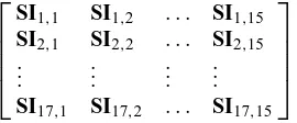
equal zero, by definition. The matrix of sustainability sub-indices for the case study scenarios can be writ-ten as follows, where the ith row represents one of the 17 crop management scenarios and the jth column represents one of the 15 sustainability sub-indices:
When PCA is applied to the portfolio of crop man-agement systems, the sustainability sub-indices were assigned individual weights or loadings on each prin-cipal component (PC). The weighting vectors are referred to as eigenvectors in PCA. The ESI can be expressed in terms of these eigenvectors as follows:
ESI=
where nc is the number of principal components re-tained, and Wi,j is the eigenvector associated with the jth principal component. The reader is referred to Sands (1995) for a more detailed discussion of the PCA analysis.
2.6.3. Temporal scale
The effect of temporal scale on the ESI was ad-dressed by varying the length of the simulation period used for the EPIC model simulations. Simulation pe-riods of 50, 100, 200 and 300 years were used for this analysis. Selection of these time frames was made in an attempt to maintain intergenerational applicability at the short end of the scale, while providing a long enough time frame at 300 years for the slower effects of soil degradation to become apparent. All EPIC sim-ulations were made with the same initial conditions and weather sequences. Therefore, the first 50 simula-tion years are identical for all time frames. The 100 to 300-year simulations all contain an identical first 100 years, and so on.
2.6.4. Uncertainty associated with model inputs
The sensitivity of the ESI to the uncertainty associ-ated with model input variables was evaluassoci-ated through sensitivity analysis. The objective of this analysis was to ascertain whether or not the ESI is more sensitive to input variability than to fundamental differences in crop management systems and/or soil types. The anal-ysis was not exhaustive in nature and did not attempt to quantify ESI sensitivity to the numerous model inputs. Rather, it attempted to characterize the ESI sensitivity using inputs to which EPIC is highly and moderately sensitive.
Model inputs for one of the 16 case study scenar-ios were varied, one at a time, while all other input variables and inputs to all other scenarios were held constant. The three variables selected for the analysis were Soil Conservation Service runoff curve number (CN), field slope (S), and initial saturated thickness of the underlying aquifer (b). These input variables were varied by positive and negative 5, 10 and 20% for the C4W2 DA crop system. The resulting changes in the ESI values for the test scenario were then compared with the other 15 scenarios whose inputs remained constant. The C4W2 DA scenario was chosen as the test scenario because of the median placement of its ESI value among the other scenarios, when computed with baseline inputs. The PCA-aggregated ESI and a 300-year time frame were used for the sensitivity analysis.
3. Result
3.1. Aggregation through PCA
Fig. 5. Component weights assigned to the 15 sustainability sub-indices through principle components analysis (PCA) for a 300-year computational time frame.
— between 0.6 and 1.1 — compared with the 11 other sub-indices. The off-site sub-indices (Li, Ri), together with GWi, received moderate weighting, in the 0.2–0.5 range. The topsoil loss sub-indices,
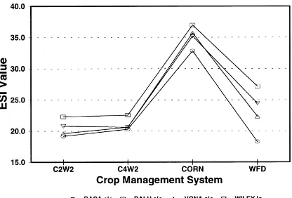
Fig. 6. ESI values for four crop management systems on four soils and four computational time frames (CORN: continuous corn; WFD: wheat-fallow, dryland; C2W2: 2-year corn, 2-year wheat rotation; C4W2: 4-year corn, 2-year wheat rotation).
TSC and TST, and one of the two organic carbon sub-indices, OCT, received the lowest weighting and hence, were the least significant in representing dif-ferences in sustainability among the case study crop management systems.
3.2. Temporal scale
agricul-tural system’s sustainability. In other words, the ESI values are not snapshots of the agricultural systems at these times — rather they integrate the agricultural system performance measures over the particular time frame.
The question of appropriate temporal scale is intrin-sic to the definition and study of sustainability. The results of this research demonstrate that the choice of temporal scale can indeed affect the nature of the in-formation obtained through use of the ESI. For all four soil types, there appears to be a less clear distinction among crop management systems with a 300-year in-dex in comparison with a 50-year inin-dex. In the Wiley and Vona soils, the systems trade places in sustainabil-ity ranking as longer time frames are considered (e.g. on the Wiley soil, the wheat-fallow system received a less sustainable ESI value than the two corn-wheat ro-tation systems out to a time frame of 200 years and re-ceived a more sustainable index value with a 300-year index). The fact that this phenomenon occurs on some but not all soils suggests that it is somehow related to soil type. Being the only non-irrigated manage-ment system, groundwater availability may also play a role in this phenomenon. Fig. 6a and c suggest that with an even longer time frame, the same phenomenon might take place on the Baca and Dalhart soils as well. Clearly, the wheat-fallow system has some advantages in the very long term, that are not fully appreciated in the short term.
3.3. Uncertainty associated with model inputs
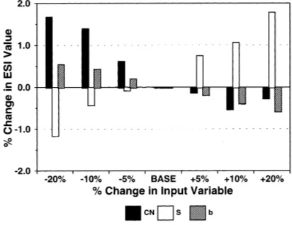
Fig. 7 presents the results of the sensitivity analysis. When CN was varied from−20 to+20% of its base value, the corresponding percent change in the ESI ranged from−0.25 to 1.7, respectively. When S was varied from−20 to +20% of its base value, the cor-responding percent change in the ESI ranged from 1.8 to−1.2, respectively. When b was varied from−20 to+20% of its base value, the corresponding percent change in the ESI ranged from−0.7 to 0.5, respec-tively.
The first two variables tested, CN and S have been found to be highly and moderately sensitive inputs, respectively, to the EPIC model. The sensitivity of the ESI, in turn, followed a similar pattern, as illustrated in Fig. 7. The effect on the ESI because of a change
Fig. 7. ESI sensitivity to three model input variables: curve number, CN, field slope, S, and initial aquifer saturated thickness, b.
in these variables was an order of magnitude smaller than the variation in the variables themselves. A 40% change in CN (the range of sensitivity tested) was re-sponsible for an approximate 2% change in ESI value. Similarly, an approximate 2.7% change in ESI value was the response to the 40% range of variation in S. The third variable tested, b, was not an EPIC input, but a parameter used in defining GW. This variable was tested because of the relatively high principle com-ponent loadings the GWC and GWT sub-indices ex-hibited (0.4 and 0.25, respectively) for the 300-year analysis. The result of the analysis was that the ESI is relatively less sensitive to changes in b, than either CN or S.
3.4. Sustainability assessment of case study portfolio
Fig. 8. ESI values from the additive aggregation scheme for 16 case study scenarios and a 50-year time frame, separated by crop man-agement system. (CORN: continuous corn; WFD: wheat-fallow, dryland; C2W2: 2-year corn, 2-year wheat rotation; C4W2: 4-year corn, 2-year wheat rotation).
where interestingly, it rates as the most sustainable system. Figs. 8 and 9 also show that the rotational systems, C2W2 and C4W2, were found to be more sustainable than the other two continuous-crop man-agement systems for all but the Baca soil. Fig. 9 shows that for all cropping systems the Dalhart sandy loam soil distinctly received an index value indicating the lowest sustainability, whereas the Baca clay loam soil received an index value indicating the highest sus-tainability. The Vona and Wiley soils received
inter-Fig. 9. ESI values from the additive aggregation scheme for 16 case study scenarios and a 50-year time frame, separated by soil type. (CORN: continuous corn; WFD: wheat-fallow, dryland; C2W2: 2-year corn, 2-year wheat rotation; C4W2: 4-year corn, 2-year wheat rotation).
mediate values, in terms of sustainability. In general, however, the degree of distinction among soil types regarding sustainability was much less pronounced than that exhibited among crop management systems.
4. Discussion
It is important to note that the ESI embodies a set of assumptions with respect to its application. The first major assumption is that of a limited or diminishing groundwater supply. This represents a constraint for agriculture that depends on the Ogallala aquifer for-mation, but not necessarily a constraint for cropping systems in other environmental regimes. Where the abundance of water or elevated water tables pose a threat to agricultural production, the nature of the GW sustainability sub-indices for the ESI require modifi-cation. Secondly, salinity is not a problem in the case study area, and no component currently exists in the ESI to account for the effect of the buildup of salts on the productivity of soil resources. Modification of the ESI would again be required where these considera-tions are important to the sustainability of agriculture. Obviously, the consideration of sustainability for any agricultural system in any environmental regime, re-quires an initial inventory of the sustaining resources, the identifying characteristics of the crop management system and their potential effect on the environment, and the evaluation of critical constraints.
Previous studies espouse inter-generational respon-sibilities for resource management because of the slow nature of degradation-induced changes in agricultural systems. Applying the ESI over time frames from 50 to 300 years demonstrated that although certain agri-cultural systems appeared to be more sustainable in the short run (50 years), these systems proved to be less sustainable when considered over longer time frames (300 years). Moreover, this phenomenon was more pronounced on some soils and less pronounced on oth-ers. These results support the notion that management practices that appear to be advantageous in the short term, may actually be less sustainable within the per-spective of a longer time frame.
Sensitivity analysis of the ESI revealed that the sen-sitivity displayed by the ESI to changes in crop man-agement system and soil type is an order of magnitude higher than its response to changes associated with the variation of selected inputs. The resulting index exhibits ample sensitivity to variations in crop man-agement practices and soil types, yet remaining sig-nificantly less sensitive to input variable uncertainty. This is an important result for the ESI because it in-dicates that the inherent variability of parameters that describe an agricultural system does not eclipse the re-sponse of the index to fundamental differences among agricultural systems.
ESI values for the 16 case study crop management systems illustrate that crop management system, rather than soil type, plays a more significant role in sustain-ability. The corn/wheat rotational systems appear to be more sustainable than either of the continuous corn or wheat systems, for all but one of the four soils studied. Results also indicate however, that no clear statement can be made concerning the role of soil type differ-entiating sustainability among the case study systems. For the 16 case study cropping systems tested, no con-sistent response was evident concerning the impact on sustainability due to differences in soil type.
The ESI was developed as a tool to gauge environ-mental sustainability based on physical, biological, and chemical processes that characterize agricultural systems. The ESI employs a modelling approach to enable relative comparisons of sustainability among a group of agricultural systems over long time frames and is thus, of little use for an individual crop manage-ment system. Although the ESI’s performed favorably, its structure — embodying only the environmental
aspects of sustainability — represents only part of the complete sustainability picture. Nevertheless, the con-cept may justify further development, especially if it could be integrated with the social and economic as-pects of sustainability.
Acknowledgements
Funding for this research was provided by the Col-orado Agricultural Experiment Station.
References
Allen, P., Van-Dusen, D., Lundy, J., Gliessman, S., 1991. Integrating social, environmental and economic issues in sustainable agriculture. Am. J. of Altern. Agric. 6 (1), 34–39. Borman, R.G., Meredith, T.S., Bryn, S.M., 1980. Geology, altitude, and depth of the bedrock surface; altitude of the watertable in 1980 and saturated thickness of the Ogallala aquifer in 1980 in the southern High Plains of Colorado. USGS Atlas HA-673, Colorado.
Brklacich, M., Bryant, C.R., Smit, B., 1991. Review and appraisal of concept of sustainable food production systems. Environ. Manage. 15 (1), 1–14.
CAST (Council for Agricultural Science and Technology), 1994. Pesticides in surface and ground water. Issue Paper No. 2. Douglass, G.K. (Ed.), 1984. Agricultural Sustainability in a
Changing World Order. Westview Press, Boulder, CO, 282 pp. Hailu, Z., Runge-Metzger, A., 1992. Calibrating a yardstick for
sustainability. Ceres, FAO Review 24 (6), 36–39.
Hansen, J.W., 1996. Is agricultural sustainability a useful concept? Agric. Syst. 50, 117–143.
Lal, R., 1991. Soil structure and sustainability. J. Sustain. Agric. 1 (4), 67–91.
Liverman, D.M., Hanson, M.E., Brown, B.J., Merideth Jr, R.W., 1988. Global sustainability: toward measurement. Environ. Manage. 12 (2), 133–143.
Neill, L.L., 1979. An evaluation of soil productivity based on root growth and water depletion. Master of Science thesis, University of Missouri Press, Columbia, MO, 348 pp.
Opie, J., 1993. Ogallala, Water for a Dry Land. University of Nebraska Press, Lincoln, NE, 412 pp.
Ott, W.R., 1978. Environmental Indices — Theory and Practice. Ann Arbor Science, Ann Arbor, MI, 371 pp.
Patil, G.P., Rao, C.R. (Eds.), 1993. Multivariate Environmental Statistics. North-Holland Series in Statistics and Probability, Vol. 6. North-Holland, New York, 596 pp.
Pierce, F.J., Larson, W.E., Dowdy, R.H., Graham, W.A.P., 1983. Productivity of soils: assessing long-term changes due to erosion. J. Soil Water Conserv. 38, 39–44.
Sands, G.R., 1995. An Environmental Sustainability Index for Agricultural Systems. Doctoral Dissertation. Department of Chemical and Bioresource Engineering, Colorado State University, Fort Collins, CO.
Senanayake, R., Sustain, J., 1991. Sustainable agriculture: defini-tions and parameters for measurement. J. Sustain. Agric. 1 (4), 7–28.
Singh, K.K., Colvin, T.S., Erbach, D.C., Mughal, A.Q., 1992. Tilth index: an approach to quantifying soil tilth. Trans. Am. Soc. Agric. Eng. 35 (6), 1777– 1785.
SCS (Soil Conservation Service), 1965. Soil Survey of Baca County, Colorado. United States Department of Agriculture, U.S. Gov. Print Office, Washington D.C.
Stein, E.C., 1992. The Environmental Sourcebook. Lyons and Burford, New York, 264 pp.
Stockle, C.O., Papendick, R.I., Saxton, K.E., Campbell, B.S., van Evert, F.K., 1994. A framework for evaluating the sustainability of agricultural production systems. Am. J. Altern. Agric. 9 (1), 45–50.
WCED (World Commission on Environment and Development), 1987. Our Common Future. Oxford University Press, New York, 383 pp.