*Tel.: 515-294-5761; fax: 515-294-0221.
E-mail address:[email protected] (G. Moschini).
Production risk and the estimation of ex-ante
cost functions
GianCarlo Moschini*
Department of Economics, Iowa State University, Ames, IA 50011-1070, USA Received 1 June 1999; accepted 25 June 2000
Abstract
Cost function estimation under production uncertainty is problematic because the relevant cost is conditional on unobservable expected output. If input demand functions are also stochastic, then a nonlinear errors-in-variables model is obtained and standard estimation procedures typically fail to attain consistency. But by exploiting the full implications of the expected pro"t maximization hypothesis that gives rise to ex-ante cost functions, it is shown that the errors-in-variables problem can be e!ectively removed, and consistent estimation of the parameters of interest achieved. A Monte Carlo experiment illustrates the advantages of the proposed procedure as well as the pitfalls of other existing estimators. ( 2001 Elsevier Science S.A. All rights reserved.
JEL classixcation: C13; C39; D24
Keywords: Cost function; Duality; Expected pro"t maximization; Nonlinear errors-in-variables; Stochastic production
1. Introduction
Following the pioneering work of Shephard (1953), Diewert (1971) and McFadden (1978), the cost function approach has proven very useful and popular in applied production studies. Insofar as the hypothesis of cost
ation is correct, estimating a cost function is usually deemed preferable to estimating a primal speci"cation of the technology because, by using input prices instead of input quantities on the right-hand side of estimating equations, one removes a potential source of simultaneous equation bias. Speci"cally, in the cost function framework input choices are modeled as a function of input prices and the output level. But, as emphasized in the recent article by Pope and Just (1996), a problem then arises when the production technology is inherently stochastic. Such a case is very important in agricultural and environmental production models, where climatic and pest factors outside of the producer's control a!ect realized output in a nontrivial fashion. When producers make their input choices prior to the resolution of this production uncertainty, the standard cost function speci"cation (which is conditional on the realized output level) is not relevant. In this setting one should instead study input choices conditional on the expected output level, i.e., estimate the structure of an
&ex-ante'cost function.
Estimating ex-ante cost functions turns out to be problematic because the expected output level that is relevant for the cost minimization problem is not observable. Pope and Just (1996) propose a solution that estimates the expected output level jointly with the cost function model, and they argue that their procedure yields consistent estimation of the parameters of the cost function. This interesting approach exploits duality to recover the form of the production function that is implied by the cost function being estimated, and then uses this production function, together with observed input quantities, to estimate the (unobserved) expected output level. But this representing unobserved expected output as a function of inputs introduces simultaneity in the speci"ed model. This simultaneity is most apparent when the cost function is equivalently represented in terms of cost-minimizing input demands, such that input quantit-ies appear as both left-hand-side variables (the dependent variables of input demand equations) and right-hand-side variables (as variables&estimating' ex-pected output). Because of this simultaneity, Pope and Just's (1996) ex-ante procedure needs to assume that expected output is a deterministic function of observed input quantities. Consequently, the proposed ex-ante estimation pro-cedure achieves consistency if input choices hold deterministically. But when input demands are stochastic (at least as far as the econometrician is concerned), as one would expect in any empirical application, the consistency property of estimates obtained from the ex-ante procedure is called into question.
models, where the relation of interest is speci"ed to hold between observable variables, in an errors-in-variables model one has a relation between unobserv-able variunobserv-ables. If the errors-in-variunobserv-ables model were linear, then one could exploit a useful equivalence between linear errors-in-variables models and linear simultaneous equations models and obtain consistent estimation procedures. Fuller (1987) provides an extensive analysis of linear errors-in-variables models. But in fact the ex-ante cost function model is inherently nonlinear. As noted by Y. Amemiya (1985), a nonlinear errors-in-variables model is not isomorphic to a simultaneous equations model, and for such nonlinear errors-in-variables models it is notoriously di$cult to obtain estimators that are consistent in the usual sense.
In this paper we provide an explicit characterization of the ex-ante cost function problem and detail the conditions that give rise to a nonlinear errors-in-variables problem. In such a setting, the ex-ante procedure leads to inconsist-ent estimates. Appeals to procedures that work in a simultaneous equations setting, such as three-stage least squares using instrumental variables, are also unlikely to produce consistent estimates. But for the stochastic production setting of interest here, however, we are able to derive a procedure that in fact yields consistent estimators. The procedure exploits the economic context that makes it interesting to estimate the ex-ante cost function, namely, expected pro"t maximization. By appealing to behavioral implications of expected pro"t maximization, we are able to e!ectively remove the errors-in-variables problem from the model. Because of its simplicity this approach is of considerable interest for a number of applications. Our claims about the inconsistency of existing estimators of the ex-ante cost function, and the consistency of our proposed procedure that exploits the implications of expected pro"t maximization, are illustrated by means of a Monte Carlo experiment. Related implications for modeling the dual structure of stochastic production are discussed.
2. The problem
1For example, only one of the many possible state-contingent outputsy
iis realized (and therefore
observed) for any one resolution of uncertainty.
consider the discrete case such that there are S states of nature, i.e.,
e3Me1, e2,2, eSN. A typical (and general) production objective for competitive
producers is expected utility maximization, which here can then be written as
max
``is the output price,w3Rn`` denotes the input price vector, and l
i3(0, 1) represents the probability of the ith state of nature (such that
+Si/1l
i"1). The utility function;(.) is assumed to be strictly increasing and
concave, thus allowing for the possibility that producers may be risk averse. Following Chambers and Quiggin (1998), a reformulation of this general production problem that exploits the notion of cost minimization takes the form
max
assuming that the state-contingent output vector (y
1,y2,2,yS) can be
produc-ed (i.e., &x3Rn` such that G(x, e
i; h0)*yi ∀i). This is what Chambers and
Quiggin (2000) call the &e!ort cost function'. Whereas c(y
1,y2,2,yS,w;h0) is
conceptually attractive, its empirical implementation is problematic.1But a use-ful simpli"cation is possible under the additional assumption of risk-neutrality (i.e.,;(.) is linear), such that the producer problem in (2) reduces to expected pro"t maximization and can be written as
max
y6 Mpy6
!C(y6,w; h)N, (4)
wherey63R
`denotes a given expected output level,his the vector of all relevant
2It is assumed thatC(y6,w;h) is strictly convex iny6, which in turns requires the expected output functiong(x;h) to be strictly concave inx. This guarantees that the solution to problem (4) is unique, if one exists.
The cost functionC(y6,w;h) is what Pope and Just (1996) call the&ex-ante cost function'. In their derivation expected pro"t maximization is postulated out-right, such that the producer problem is written as
max
x
ME[pG(x,e; h0)!w)x]N, (6)
where E is the mathematical expectation operator (which is de"ned over the distribution of the random variablee). By de"ning an&expected output'function as g(x; h),E[G(x, e; h0)], where h is the vector of all relevant parameters (which here include parameters of the distribution of the random variablee), this expected pro"t maximization problem can be equivalently expressed in terms of two distinct problems. First, the producer chooses the optimal input vector to produce a given level of expected output, that is (s)he solves
min
x
Mw)xDy6)g(x; h)N. (7)
Let xH"h(y6,w;h) denote the solution to problem (7). Then the ex-ante cost function is de"ned asC(y6,w;h),w)h(y6,w;h). Given the optimal input choices
summarized by C(y6,w;h), the second step is for the producer to choose the optimal level of expected output that maximizes expected pro"t, that is to solve the program in Eq. (4).2
Note that the ex-ante cost function C(y6,w; h), by construction, re#ects the producers' expectations in addition to the technological properties of the stochastic production function. For example, changes in the producers'beliefs about the distribution of the random variableewould a!ect the structure of this ex-ante cost function. Hence, any empirical speci"cation of the ex-ante cost function is bound to represent, in some sense, a reduce-form function whose meaning is somewhat di!erent from what one ascribes, from duality, to standard cost functions. But C(y6,w;h) here does describe a relevant cost minimization behavior in a parsimonious way, and therefore it is often of considerable interest to estimate its parameters. Unfortunately,C(y6,w;h) is conditional on expected (or planned) outputy6, which is not observable, and hence direct estimation of the ex-ante cost function is not feasible.
3. Ex-ante cost function estimation
3Regularity conditions include thatg(x;h) be quasi-concave inx, which is guaranteed by the assumed curvature conditions for expected pro"t maximization [i.e.,g(x;h) is concave]. data) have simply ignored the problem. That is, researchers have routinely estimatedC(y, w; h), whereyis the observed (ex-post or realized) output, when in fact they should have been estimatingC(y6,w; h). This approach, which is here labeled as the &standard' approach, essentially uses observed outputy as the proxy for the unobserved expected outputy6. But becausey&measures'the true variabley6 only with error, namKve (least-square) type estimators that ignore this problem lead to inconsistent estimates.
To overcome the inconsistency of the standard cost function approach when production is stochastic, Pope and Just (1996) propose an alternative and original estimation procedure which entails estimating y6 simultaneously with the ex-ante cost function. First, recall that ify6 were observable the parameters
hcould be estimated e$ciently by"tting the system ofninput demand functions
h(y6, w;h), which by Shephard's lemma are related to the ex-ante cost function by
h(y6, w;h),+
wC(y6,w; h). But becausey6 is not observable, Pope and Just (1996)
propose to replace it by the output level which solves
max
y6
G
y6
K
minw
[1!C(y6, w; h)#w)x]*1
H
. (8)Denote such a solution byy60. Under standard regularity conditions, by duality theory it must then be thaty60,g(x; h).3Hence, this method reduces to estima-ting the set of input demand equations withy6 replaced by the expected output functiong(x;h). Although this point was perhaps not emphasized enough, it was certainly articulated explicitly by Pope and Just (1996) (e.g., in the"rst unnum-bered equation on p. 240). With such a substitution, to allow input demands to be stochastic one would need to write the system of input demand equations as
x"h(g(x,h), w;h)#e, (9)
whereeis the error vector of input demands.
4Again, if the form ofg(.) that is consistent with the parameterization ofC(.) is not known, theng(.) can be retrieved numerically.
this is due to the fact that with (9) one is trying to estimate a cost function without observing output, which means that Eqs. (9) de"ne a simultaneous equation system that is not identi"ed. To overcome this problem Pope and Just (1996, p. 240) suggest adding an equation to the estimating system. In our notation, one would then estimate a system of n#1 equations given by the
ninput demand equations in (9) plus the production function equation, that is,4
y"g(x; h)#u, (10)
where u is an error term induced by the random variable e (i.e., u, y!E[G(x, e; h)]).
If the functional speci"cation is such that the parameter vector h is now identi"ed, then the system of equations (9) and (10) can be used to estimate this parameter vector. But although joint estimation of Eqs. (9) and (10) is in principle possible, it is now apparent that there is still a major unresolved issue in this setting. Speci"cally, the system ofn#1 equations in (9) and (10) entails that the (possibly stochastic) vector of input quantities x appears on the right-hand side of all equations. This simultaneity feature was not explicitly discussed in Pope and Just (1996). Clearly, if input choices hold deterministically (such that e,0 in Eqs. (9)), then their proposed estimation procedure will produce consistent estimates of the underlying parameters. But if one were to allow for the realistic feature of errors in input demands, the ex-ante procedure is unlikely to yield consistent estimates.
Recognizing that simultaneous equation bias might be a problem if input demands are allowed to be stochastic has led Pope and Just (1998) to implement, in a related setting, a three-stage least-squares estimation procedure that uses instrumental variables (IV). But whether or not such an&IV ex-ante'approach leads to consistent estimates is an open question because, for reasonable
speci-"cations of the stochastic nature of input demands, the simultaneous equations representation of (9) and (10) is not the appropriate one. Rather, when both production and input demands are stochastic, the model that is obtained is likely to give rise to an errors-in-variables problem. Because the model is also inherently nonlinear, estimation techniques that yield consistent estimators for simultaneous equation models do not typically work here (Y. Amemiya, 1985; Hsiao, 1989).
4. Stochastic input demands and the errors-in-variables problem
To gain more insights into this problem it is necessary to be precise about the source of these error terms. Here we analyze in detail what McElroy (1987) has called the &additive generalized error model' (AGEM). This rationalization provides an attractive and coherent explanation for stochastic input demands, and for this reason was advocated explicitly in Pope and Just's (1996, 1998) empirical applications. Speci"cally, producers are assumed to minimize cost conditional on a production function which, in our setting, can be written as
g(x!e; h), where the vector eis parametrically known to producers. Hence, optimal input choices are written as
x"h(y6, w; h)#e (11)
with total production costsC,w)x given by
C"C(y6, w; h)#w)e. (12)
By assuming that the vector e, while parametrically known to producers, is unobservable to the econometrician, the deterministic input demand setting at the producer level translates naturally into an internally consistent stochastic input demand setting for the purpose of estimation (McElroy, 1987).
Although clearly appealing from an economic point of view, the AGEM rationalization for stochastic input demands, in conjunction with the assumed stochastic production structure, turns out to create a problem for the ex-ante estimation procedure. Speci"cally, although one can"nd the expected output functiong(. ;h) dual to the cost function being used [by solving (8), say], the argument of this function that is relevant for the purpose of computing expected outputy6 cannot be observed. In other words, if we de"nex6,x!e, then the (n#1) equation system of input demands and production function implied by the AGEM model is
x"h(g(x6;h),w;h)#e, (13)
y"g(x6, h)#u, (14)
where g(x6,h),y6. Clearly, the system of equations (13) and (14) cannot be estimated directly because x6 is not observed. Indeed, the problem here is completely analogous to the one that we have set out to solve [i.e., estimating
C(y6, w; h) wheny6 is not observed]. Thus, with stochastic input demands and stochastic production, the estimating equations for the ex-ante cost model belong to the class of nonlinear errors-in-variables models. As mentioned earlier, such models are conceptually distinct from simultaneous equation models, and the estimators that apply to the latter do not typically work for the former (Y. Amemiya, 1985).
5Of course, here realized output can be written as a function of observed inputs, because in this case input errors are productive. Hence,y"g8(x,hI)#u, whereg8(x;hI),E[G(x,e;h0)] (this expecta-tion operator is de"ned only over the random variable e, and hence the vectorhI di!ers from
hbecause it includes parameters of the distribution ofebut not ofe). But writingy"g8(x,hI)#uis not very useful in estimating the ex-ante cost function because it isg(x6;h), and notg8(x;hI), which in this setting is dual toC(y6,w;h).
errors-in-variables model. Other internally consistent rationalizations for the stochastic terms of input demands can yield an errors-in-variables problem when stochastic input demands are combined with a stochastic output. Con-sider, for example, the following alternative rationalization for stochastic input demands: agents make decision errors. To steer clear of making inconsistent assumptions we need to be explicit about the decision framework. In particular, the assumption here is that there are&input errors'that cannot be avoided, but producers are aware that such errors will be committed and they know the distribution of these errors. This is equivalent to saying that producers choosex6, say, but the choicex"x6#eis implemented, whereedenotes a vector of input demand errors satisfying E[e]"0. Of course,x6 is not observable whereasxis observed. But once x is implemented, it is x which enters the production function (in other words, input errors here are&productive').
Speci"cally, the production function is written as G(x,e; h0),G(x6# e,e; h0), and the expected pro"t maximization problem can be written as
max
x6
ME[pG(x6#e, e;h0)!w)(x6#e)]N, (15)
where the expectation operator E is here de"ned over the distribution of the random variableseande. In this setting the relevant expected output function is
g(x6;h),E[G(x6#e,e; h0)], where again the expectation operator E is de"ned over the distribution of Me,eN, and his the vector of all relevant parameters (which here include the parameters of the distributions ofMe, eN). The ex-ante cost function dual to the expected output function is therefore de"ned as
C(y6,w; h),min
x6
Mw)x6 Dy6)g(x6; h)N (16)
and the expected pro"t maximization problem in (15) can then be stated as the program in (4). In this setting the stochastic input demands equations can be written as x"h(y6, w; h)#e, where by Shephard's lemma h(y6,w; h), +
wC(y6, w;h). As before, these demand functions cannot be estimated directly
6Of course, ife,0 the system ofninput demands would have to hold deterministically, whereas ifu,0 then the output equation would need to hold deterministically. Hence such cases are somewhat uninteresting from an empirical point of view.
Based on the foregoing, it is apparent that allowing for stochastic input demands introduces subtle issues for the interpretation and estimation of the ex-ante cost function. Recall that the hallmark of this approach is to exploit duality to recover the expected output function dual to the adopted speci"cation of the ex-ante cost function. But duality relies crucially on the assumed optimiz-ing behavior of producers, and the dual form that one recovers can only re#ect the optimizing choices of producers. If the identity between observed input quantities and optimal producer choices is broken, by allowing stochastic terms in input demands, the internal consistency of the proposed ex-ante procedure is a!ected. The preceding structural explanations of input demands make it clear that the ex-ante procedure does apply in a special case, that of nonstochastic input demands. If input demands do not have error terms (e,0), then x"x6
and the ex-ante procedure e!ectively removes the errors-in-variables problem (while still allowing for stochastic production). Similarly, our discussion also identi"es the other special case that arises when production is not stochastic (u,0). In this case, which is implicitly assumed in most existing empirical applications, one hasy"y6 and the errors-in-variables problem disappears from the cost model (while still allowing for stochastic input demands).6But with the joint presence of error terms in input demand equations and in the production equation, exploiting duality does not eliminate&unobserved'variables and the ex-ante cost model is still a!ected by an errors-in-variables problem.
5. A&full information'solution
Fortunately, an alternative procedure to estimate the ex-ante cost function suggests itself in the context of the economic problem where the ex-ante cost function is relevant. Speci"cally, recall that interest in the ex-ante cost function
C(y6, w; h) is motivated here by the assumption that producers solve the expected pro"t maximization problem in Eq. (6). Because this expected pro"t maximiza-tion problem can equivalently be written as (4), then from the optimality condition of problem (4) one "nds the solution y6H"s(p, w; h), where the parametric structure of th ex-ante supply functions(p, w; h) is implied by the structure of the ex-ante cost functionC(y6, w; h). This optimal expected produc-tion level depends on the (exogenously given) output pricep. If such an output price is observable (as it is usually the case) then p provides the obvious
&instrument' for the unobserved expected output, and the function s(p, w;h) provides the correct nonlinear mapping for this instrument. Thus, in this setting one can estimate the parameters of the cost function by "tting the system of
ninput demand equations:
x"h(s(p, w;h),w;h)#e. (17)
If so desired, the system of input demand functions in (17) can be supple-mented by the expected output function equation, that is
y"s(p, w;h)#u. (18)
Note, however, that here Eq. (18) is not necessary in order to identify all the parameters of the model. Unlike the ex-ante input demand system in (9), the system in (17) typically allows for the estimation of all cost parameters (again this is made possible by the presence of the output pricep).
The approach that we have suggested, based on the expected pro"t maximiza-tion problem actually solved by the producer, will yield consistent estimates of the parameters of the underlying technology because it e!ectively removes the errors-in-variables problem. It bears repeating that our proposed approach does not require additional assumptions relative to those inherent in the setting being analyzed. Speci"cally, the hypothesis of expected pro"t maximization is already made to motivate interest in the ex-ante cost function; and, given that, the shape of the ex-ante supply functions(p, w;h) is fully determined by the cost function
6. A Monte Carlo illustration:The generalized CES model
To illustrate the properties of the alternative estimators for the ex-ante cost function, we have constructed a Monte Carlo experiment that carefully repres-ents all the features of the problem being analyzed. For this purpose, we work with a cost function that admits a closed form solution for the dual production function. Hence, we can avoid the complications of retrieving this function numerically as part of the estimation routine, a computational task that featured prominently in Pope and Just (1996) but which is peripheral to the main issue analyzed here. Speci"cally, we consider a generalized constant elasticity of substitution (CES) cost function that allows for decreasing returns to scale (such that it can be consistent with the expected pro"t maximization problem that has been used to motivate the ex-ante cost function).
6.1. Experiment design
The AGEM speci"cation of this CES cost function is written as
C"y6b
A
+nconstant Allen-Uzawa elasticity of substitution between inputs. The parameter
b controls the curvature of the cost function in y6, and the condition b'1 ensures that the cost function is (strictly) convex iny6. From Shephard's lemma, input demands consistent with this cost function are
x
Consistent with the AGEM speci"cation, the terms e
i are parametrically
known to the producers but are treated as random variables by the econo-metrician. Hence, the parameter vector to be estimated ish,(a, b,p). For this particular cost function it is veri"ed that the (expected) production function [i.e., the solution to problem (8)] can be derived explicitly as
g(x!e; h)"
A
+nHence, Eq. (21) here can be used to implement the ex-ante methods discussed earlier.
7Given the normalizations chosen for the exogenous variables, the mean ofx
iis approximately
equal toaiand the mean ofyis equal to one. they will choose the level of expected output
s(p,w; h)"
A
pHence, the supply function in (22) here can be used to implement our proposed method based on expected pro"t maximization.
Now the Monte Carlo experiment proceeds as follows.
A. First, we choose the number of inputs to be four (i.e.,n"4), and we set the true values of the parameters as follows:
a1"0.1,a2"0.2,a3"0.3,a4"0.4,b"1.2,p"0.5.
B. Next, we choose the design matrix of exogenous variables (the vectors of expected outputy6 and of input pricesw), which is then held"xed through-out. Here we use an initial sample of 25 observations taken from a recent application using agricultural data (see the appendix for more details). All variables are normalized to equal unity at their sample mean.
C. For each replicationj"1,2,J, we construct a pseudo-sample of optimal
input quantities by using Eqs. (20), with the vectoregenerated as N(0,X). Similarly, for each replication we construct a pseudo-sample of stochastic output asy"y6#u, where the random termuis generated as N(0,/2). The standard deviation of each random variable was set to 10% of the corre-sponding mean.7Thus, for the output stochastic term we set/"0.1. For the covariance matrix of the terms e
i we consider three cases: one with
independent input demand errors (X
0), one with such errors being
negative-ly correlated (X1) and one with these input errors being positively correlated (X2). Speci"cally, the three covariance matrices for the vector e that we consider are
8For each draw we checked the regularity conditions (x
i!ei)'0, which turned out to be always
satis"ed.
9We rely on four primitive instrumental variables: three input prices (de#ated by the fourth input price) and the output price (de#ated by the fourth input price). We use the four primitive variables plus their squares and cross-products that, together with a constant, give a total of 15 instruments that are used in the IV procedure.
10Consistent with the assumption of expected pro"t maximization under competition and stochastic production, the price series used in the Monte Carlo experiment was generated as
p"C
y6(y6,w;h), whereCy6(y6,w;h) is readily obtained from the CES cost function speci"cation in the text. Note that this output price series is used by both the IV ex-ante approach and by our proposed procedure.
antithetic counterparts.8For each sample,"ve models are estimated: (i) The true model consisting of four input equations in (20). The results
from this model provide a useful benchmark for evaluating the feasible estimators.
(ii) The standard model, which is the same as the true model but with
yreplacingy6.
(iii) The ex-ante procedure suggested by Pope and Just (1996), consisting of
"ve equations [four input equations and the output equation with the structure of Eqs. (9) and (10)], that is
x (iv) The&IV ex-ante'procedure suggested by Pope and Just (1998), which estimates Eqs. (23) and (24) by nonlinear three-stage least squares using a set of instrumental variables (which includes output pricep).9
(v) The new approach proposed in this paper, which uses the ex-ante supply functions(p,w; h) in lieu of the unobserved expected outputy6.10
Because this approach relies on the implications of expected pro"t maximization, it is labeled&max E[P]'. Hence, here we"t the following system of four input demand equations plus the output equation:
11Note that the"rst two methods entailM"4, whereas for the last three methodsM"5.
12Thus, this yields what is usually referred to as the nonlinear three-stage least-squares estimator (e.g., T. Amemiya, 1985). As mentioned earlier, hereq"15.
13Because+ni
/1ai"1, only threeaiparameters need to be estimated.
6.2. Estimation
Each of the alternatives entails estimating a system of M equations using
¹ observations.11 Thus, for each alternative the model can be written as >"f(Z,h)#l, where y is the ¹M]1 stacked vector of the left-hand-side variables,f(.) is a nonlinear (vector valued) function,Zis the (stacked)¹M]K
matrix of all right-hand-side variables, his the vector of all parameters to be estimated and l is the ¹M]1 stacked residual vector. The error terms are assumed to be contemporaneously correlated but serially independent, that is, E[ll@]"W?I
T, where W is the M]M contemporaneous covariance matrix
andI
Tis the identity matrix of order¹. For four of the models considered (true,
standard, ex-ante and our new procedure) the system of interest is treated as a standard nonlinear seemingly unrelated regression model. Iterated minimum distance estimation is used (which converges to the maximum likelihood es-timator). Speci"cally, at each iteration stage the vector of parameters is found by minimizing
(>!f(Z,h))@(W~1?I
T)(>!f(Z,h)),
where W is the current estimate of the contemporaneous covariance matrix, which is updated at each iteration step until convergence. For the IV ex-ante model, on the other hand, at each iteration the vector of parameters is found by minimizing
(>!f(Z,h))@(W~1?(=(=@=)~1=@))(>!f(Z,h)),
where=is the¹]qmatrix of all instrumental variables, and again the estimate of the contemporaneous covariance matrixWis updated at each iteration step until convergence.12
6.3. Results
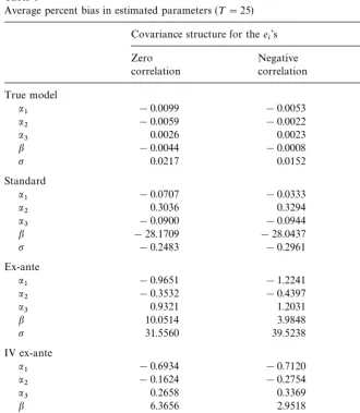
The results are summarized in Tables 1}4. Table 1 reports the average percent bias for each parameter, for each estimation method and for all three covariance structures considered.13Average percent bias is computed as
1
J J + j/1
A
hKji!h i h
i
B
Table 1
Average percent bias in estimated parameters (¹"25) Covariance structure for thee
i's
Zero Negative Positive
correlation correlation correlation
True model
a
1 !0.0099 !0.0053 !0.0076
a2 !0.0059 !0.0022 !0.0038
a3 0.0026 0.0023 0.0014
b !0.0044 !0.0008 !0.0106
p 0.0217 0.0152 0.0133
Standard
a
1 !0.0707 !0.0333 !0.0967
a
2 0.3036 0.3294 0.2829
a3 !0.0900 !0.0944 !0.0892
b !28.1709 !28.0437 !28.2886
p !0.2483 !0.2961 !0.1942
Ex-ante
a1 !0.9651 !1.2241 !0.6876
a
2 !0.3532 !0.4397 !0.2513
a
3 0.9321 1.2031 0.6587
b 10.0514 3.9848 15.8727
p 31.5560 39.5238 22.9752
IV ex-ante
a1 !0.6934 !0.7120 !0.6318
a2 !0.1624 !0.2754 !0.0575
a3 0.2658 0.3369 0.1881
b 6.3656 2.9518 9.7748
p 18.8045 23.6668 13.5399
max E[P]
a1 0.0001 0.0054 !0.0011
a2 0.0004 0.0019 !0.0004
a3 0.0039 !0.0003 0.0030
b 0.0023 0.0005 0.0036
p !0.0932 !0.0273 !0.0714
wherehKjiis the estimatedith parameter in thejth replication. All"ve methods do a reasonably good job at estimating the mean parameters a
i. Also, the new
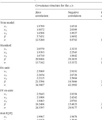
Table 2
Percent RMSE in estimated parameters (¹"25)
Covariance structure for thee i's
Zero Negative Positive
correlation correlation correlation
True model
a
1 1.9789 1.6518 1.7121
a2 1.8872 2.0389 1.5723
a3 1.6508 1.8927 1.3787
b 5.7451 1.8892 7.8247
p 12.5260 8.8782 11.0176
Standard
a1 2.0570 2.3233 1.7462
a2 1.9383 2.2543 1.6151
a3 1.6710 1.8842 1.4034
b 29.9088 29.3855 30.4255
p 13.7342 15.3372 11.7556
Ex-ante
a
1 2.5069 2.9191 2.0513
a
2 2.2654 2.6728 1.8754
a
3 2.2115 2.5664 1.7860
b 21.3586 16.5466 26.4365
p 34.3807 42.1902 25.8993
IV ex-ante
a1 2.5643 2.8354 2.2131
a2 2.1008 2.4242 1.7613
a3 1.8463 2.0761 1.5461
b 18.2406 15.4823 21.0803
p 24.3597 28.9177 19.4645
max E[P]
a1 1.9967 1.9478 1.6973
a2 1.6915 1.2049 1.4824
a3 1.5558 1.2857 1.3435
b 0.1681 0.0676 0.2095
p 11.7455 7.8556 10.8120
does a better job than the standard model at estimating this scale parameter, although the estimatedb is a!ected by considerable bias in this case as well. Furthermore, this ex-ante model provides a much more biased estimator for the elasticity of substitution p (for example, for the case of uncorrelated e
i, the
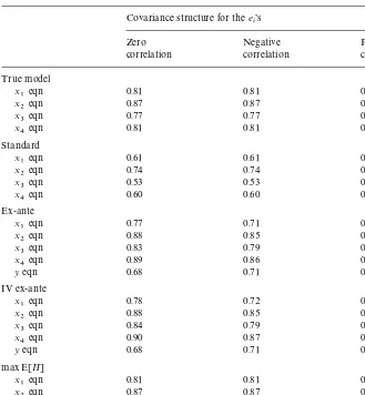
Table 3
AverageR2of estimated equations (¹"25)
Covariance structure for thee
14The performance of the IV estimator could be improved by the bias adjustment method proposed by Amemiya (1990). But such a computationally intensive method still does not lead to consistency, and in our context is bound to be inferior to the procedure we are proposing. approach, although estimates are still a!ected by considerable bias.14 As ex-pected, changing the correlation structure of thee
i does not a!ect the
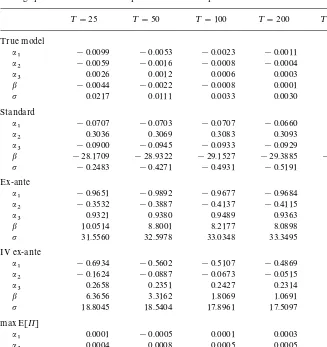
Table 4
Average percent bias in estimated parameters and sample size
¹"25 ¹"50 ¹"100 ¹"200 ¹"400
a3 0.0026 0.0012 0.0006 0.0003 0.0001
b !0.0044 !0.0022 !0.0008 0.0001 !0.0004
p 0.0217 0.0111 0.0033 0.0030 0.0005
Standard
a1 !0.0707 !0.0703 !0.0707 !0.0660 !0.0705
a2 0.3036 0.3069 0.3083 0.3093 0.3110
a3 !0.0900 !0.0945 !0.0933 !0.0929 !0.0990
a3 0.9321 0.9380 0.9489 0.9363 0.9295
b 10.0514 8.8001 8.2177 8.0898 7.9065
p 31.5560 32.5978 33.0348 33.3495 33.3922
IV ex-ante
a
1 !0.6934 !0.5602 !0.5107 !0.4869 !0.4622
a2 !0.1624 !0.0887 !0.0673 !0.0515 !0.0400
a3 0.2658 0.2351 0.2427 0.2314 0.2196
b 6.3656 3.3162 1.8069 1.0691 0.6704
p 18.8045 18.5404 17.8961 17.5097 17.2222
max E[P]
a1 0.0001 !0.0005 0.0001 0.0003 0.0000
a2 0.0004 0.0008 0.0005 0.0005 0.0000
a3 0.0039 0.0009 0.0003 0.0001 0.0001
b 0.0023 0.0012 0.0005 0.0003 0.0001
p !0.0932 !0.0276 !0.0172 !0.0088 !0.0041
the e
i does a!ect the performance of the ex-ante procedure; with positively
correlated e
i the bias in the scale parameter gets larger and the bias in the
elasticity of substitution gets smaller, whereas the opposite holds true for negatively correlatede
i.
The conclusions based on the average percent bias of Table 1 are supported by the average percent root mean square errors (RMSE) reported in Table 2. The entries of this table are computed as J1/J+Jj/1([(hKji!h
i)/hi]100)2, and
Table 3 reports the averageR2, over all replications, for each equation in each estimation method. Speci"cally, theR2for each equation is de"ned as the square of the correlation coe$cient between observed and"tted left-hand-side variable. This table provides an ex-post check on the signal-to-noise ratio that we have implemented in our Monte Carlo experiment. Note that the&"t'of the various models is similar to that of many empirical applications. Indeed, in some sense our experiment has been conservative in that the magnitude of the production error that we have used is relatively large compared with the magnitude of the input demand errors (thus, our setup is somewhat slanted in favor of both ex-ante procedures relative to the standard procedure).
Finally, Table 4 illustrates the"nite-sample properties of the"ve estimators considered as the sample size increases. Speci"cally, to get an idea of the asymptotic convergence of the various estimators we allow the sample size to increase from 25 to 400 (each time we double the design matrix, such that the exogenous variables are multiple repeats of those reported in the appendix). For the true model and our proposed model it is clear that the small-sample bias converges to zero as the sample size is increased. On the other hand, for the standard model, for the ex-ante procedure, and for the IV ex-ante method, the bias does not seem to be in#uenced by the increasing sample size. In particular, it is clear that the ex-ante procedure leads to inconsistent parameter estimates. Indeed, the ex-ante procedure arguably produces worse results than the standard approach. Of course, the ranking of these two inconsistent estimators likely depends on the magnitude of the randomness of the production function relative to the randomness of the input demand functions (recall that the errors-in-variables problem is due touin the standard model, whereas it is due toein the ex-ante procedure).
7. Further discussion
The results of our Monte Carlo experiment provide a compelling example of the deleterious consequences of ignoring production risk when estimating a cost function. Indeed, these results are a bit more general in that it is not even necessary to postulate production risk (in addition to input demand errors) in order to obtain an errors-in-variables cost function model. The above setting would in fact be unchanged if no production risk were present, but the error termuarose in a manner similar to thee
i, i.e., from an AGEM rationalization.
In other words, one could postulate that the pro"t-maximizing agents have a production function written asy"g(x!e;h)#u, where the termseanduare known to the producer but unobservable to the econometrician. De"ning
(and realistic) class of problems than that of production uncertainty. But regardless of the source of the production erroru, the approach that we have suggested, based on the expected pro"t maximization problem actually solved by producers, yields consistent estimates of the parameters of the underlying technology.
As mentioned earlier, a practical problem is that for many#exible speci" ca-tions of C(y6, w;h) one cannot solve explicitly for the ex-ante supply function
s(p, w, h). In such a case one could numerically retrieves(p,w, h) as part of the estimation routine. Alternatively one can recognize that, in this context, it is better to specify and estimate an expected pro"t function rather than an ex-ante cost function. Speci"cally, if the value function of problem (6) is written as
P(p, w;h), then under standard assumptions this expected pro"t function exists and is continuous, linearly homogeneous and convex in (p,w). This expected pro"t function is completely analogous to the standard pro"t function that obtains under conditions of certainty (as analyzed, for example, by Lau, 1976). Thus, instead of specifying an ex-ante cost functionC(y6, w;h), under production uncertainty the analysis can proceed by specifying the parametric structure of the expected pro"t function P(p, w;h). By Hotelling's lemma, this implies a coherent structure for the output supply functions(p, w; h)"P
p(p, w;h) and
the vector of input demand functions x(p,w; h)"!+
wP(p,w; h), where x(p,w; h),h(s(p, w;h),w; h). Hence, from a proper parametric speci"cation of
P(p, w;h) (say, Lau's (1974) normalized quadratic model), one can derive a coherent set of output supply and input demand equations that can be used in estimation. Because this route essentially removes the errors-in-variables prob-lem, estimation of this set of equations produces consistent estimates of all the underlying parameters that are identi"ed. If interest centers explicitly on the properties of the ex-ante cost function, then one can exploit duality to retrieve the latter (numerically or analytically) from the expected pro"t function, i.e., by solving
C(y6,w; h)"max
p
Mpy6!P(p, w; h)N. (27)
15For example, as noted by Pope and Just (1996), in our setting output price can also be allowed to be a random variable providedpandeare independently distributed. But then the relevant output price for producers'decision is the expected pricep6,E[p]. Ifp6 is observed (say, a futures price), the analysis of this paper carries through directly. Ifp6 is not observed, on the other hand, then the procedure proposed here needs to be augmented by a model specifying howp6 is formed, say by postulating&rational expectations'[see Pesaran (1987) for a comprehensive introduction]. broader setting.15 But more generally, when price and production risks are unrestricted and/or decision makers are risk averse, the cost functionC(y6,w;h) may not be of much interest anyway and, as discussed earlier in Section 2, one may need to revert to more general cost function concepts.
8. Conclusion
Under production risk a likely object of interest in production studies is the ex-ante cost function, as noted by Pope and Just (1996). But when input demand equations (in addition to the production function) are also genuinely stochastic, the ex-ante procedure is unlikely to improve over the standard estimation procedure because it does not solve the fundamental problem that arises in this context, i.e., the ex-ante cost model inevitably leads to a nonlinear errors-in-variables problem. It is notoriously di$cult to obtain consistent estimators for this class of models. For the particular case of an ex-ante cost function that naturally arises in the context of the expected pro"t maximization hypothesis, however, we have shown that it is possible to achieve consistent estimation for the parameters of the ex-ante cost function. Speci"cally, by exploiting the full implications of the expected pro"t maximization hypothesis one can e!ectively remove the errors-in-variables problem. The results of a carefully structured Monte Carlo experiment provide support for our claim about the properties of various estimation procedures. In particular, our proposed procedure to esti-mate the ex-ante cost function yields estiesti-mates of the underlying technological parameters that are equivalent to those of the (unfeasible) true model.
Acknowledgements
This is Journal Paper No. J-18316 of Iowa Agriculture and Home Economics Experiment Station, Project No. 3539. The author thanks Y. Amemiya, R. Chambers, D. Hennessy, H. Lapan, S. Lence, P.L. Rizzi and the Journal's anonymous reviewers for helpful comments.
Appendix
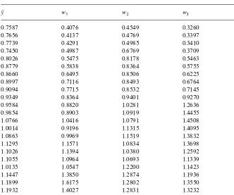
Table 5
Data used in the Monte Carlo experiment
y6 w
1 w2 w3 w4
0.7587 0.4076 0.4549 0.3260 0.4446
0.7656 0.4137 0.4769 0.3397 0.4093
0.7739 0.4291 0.4985 0.3410 0.4176
0.7450 0.4987 0.6769 0.3709 0.4384
0.8026 0.5475 0.8178 0.5463 0.4042
0.8779 0.5838 0.8364 0.5755 0.3460
0.8660 0.6495 0.8506 0.6225 0.5161
0.8997 0.7116 0.8493 0.6764 0.6261
0.9094 0.7715 0.8532 0.7145 0.6713
0.9349 0.8364 0.9401 0.9270 0.8419
0.9584 0.8820 1.0281 1.2636 1.1237
0.9854 0.8903 1.0919 1.4455 1.4533
1.0766 1.0416 1.0791 1.4508 1.6860
1.0014 0.9196 1.1315 1.4095 1.6439
1.0863 0.9969 1.1519 1.3832 1.8139
1.1295 1.1571 1.0834 1.3698 1.4502
1.1026 1.1394 1.0380 1.2592 1.2138
1.1055 1.0964 1.0693 1.1339 1.3617
1.0135 1.0547 1.2200 1.1423 1.2031
1.1447 1.3850 1.2874 1.1936 1.1098
1.1899 1.6175 1.2802 1.3550 1.1115
1.1932 1.6027 1.2831 1.3232 1.1237
1.1965 1.6334 1.2936 1.2816 1.2083
1.2147 1.8553 1.3301 1.2958 1.0642
1.2684 1.8786 1.3777 1.2534 1.3174
take four input price series from their data: labor (w
1), materials (w2), energy
(w
3) and capital (w4). The aggregation of input prices in these four categories has
been very common in the applied literature [leading to the so-called&KLEM'
models; see Berndt and Wood (1975) for an early example]. Variables w
1,
w
3 and w4 are reported directly by Ball et al. (1997), whereas w2 had to be
computed from the three nonenergy intermediate input price series that they report. We did so by using Fisher's ideal index formula (with mean values over the entire period as the base). The expected output seriesy6 was generated as the
References
Amemiya, T., 1985. Advanced Econometrics. Harvard University Press, Cambridge, MA. Amemiya, Y., 1985. Instrumental variable estimator for the nonlinear errors-in-variables model.
Journal of Econometrics 28, 273}289.
Amemiya, Y., 1990. Two-state instrumental variable estimators for the nonlinear errors-in-variables model. Journal of Econometrics 44, 311}332.
Ball, V.E., Bureau, J.-C., Nerhing, R., Somwaru, A., 1997. Agricultural productivity revisited. American Journal of Agricultural Economics 79, 1045}1064.
Berndt, E.R., Wood, D.O., 1975. Technology, prices, and the derived demand for energy. Review of Economic and Statistics 57, 259}268.
Chambers, R.G., Quiggin, J., 1998. Cost functions and duality for stochastic technologies. American Journal of Agricultural Economics 80, 288}295.
Chambers, R.G., Quiggin, J., 2000. Uncertainty, Production, Choice and Agency: The State-Contingent Approach. Cambridge University Press, New York, NY.
Diewert, W.E., 1971. An application of the Shephard's duality theorem: a generalized Leontief production function. Journal of Political Economy 79, 481}507.
Fuller, W.A., 1987. Measurement Error Models. Wiley, New York, NY.
Hausman, J.A., Newey, W.K., Hichimura, H., Powell, J.L., 1991. Identi"cation and estimation of polynomial errors-in-variables models. Journal of Econometrics 50, 273}295.
Hausman, J.A., Newey, W.K., Powell, J.L., 1996. Nonlinear errors-in-variables estimation of some Engel curves. Journal of Econometrics 65, 205}233.
Hsiao, C., 1989. Consistent estimation for some nonlinear errors-in-variables models. Journal of Econometrics 41, 159}185.
Lau, L., 1974. Applications of duality theory: a comment. In: Intriligator, M.D., Kendricks, D.A. (Eds.), Frontiers in Quantitative Economics, Vol. II. North-Holland, Amsterdam, pp. 176}199. Lau, L., 1976. A characterization of the normalized restricted pro"t function. Journal of Economic
Theory 12, 131}163.
McElroy, M., 1987. Additive general error models for production, cost, and derived demand or share systems. Journal of Political Economy 95, 737}757.
McFadden, D., 1978. Cost, revenue, and pro"t functions.. In: Fuss, M., McFadden, D. (Eds.), Production Economics: A Dual Approach to Theory and Applications, Vol. I. North-Holland, Amsterdam, pp. 3}109.
Pesaran, M.H., 1987. The Limits to Rational Expectations. Blackwell, Oxford, UK.
Pope, R.D., Just, R.E., 1996. Empirical implementation of ex-ante cost functions. Journal of Econometrics 72, 231}249.
Pope, R.D., Just, R.E., 1998. Cost function estimation under risk aversion. American Journal of Agricultural Economics 80, 296}302.