Probability And Statistics For Engineers (3)

(1)

Scilab Textbook Companion for

Probability And Statistics For Engineers And

Scientists

by S. M. Ross

1 Created by

Deeksha Sinha

Dual Degree

Electrical Engineering

IIT Bombay

College Teacher

None

Cross-Checked by

Mukul R. Kulkarni

August 10, 2013

(2)

Book Description

Title: Probability And Statistics For Engineers And Scientists

Author: S. M. Ross

Publisher: Elsevier, New Delhi

Edition: 3

Year: 2005

(3)

Scilab numbering policy used in this document and the relation to the above book.

Exa Example (Solved example)

Eqn Equation (Particular equation of the above book)

AP Appendix to Example(Scilab Code that is an Appednix to a particular Example of the above book)

(4)

List of Figures

2.1 pie chart . . . 12

9.1 Scatter Diagram. . . 76

9.2 Relative humidity and moisture content. . . 77

9.3 Moisture against Density . . . 78

9.4 Regression to the mean . . . 82

9.5 Percentage of chemical used . . . 88

9.6 Percentage of chemical used . . . 88

9.7 Polynomial Fitting . . . 91

13.1 determining control limits . . . 124

13.2 determining control limits . . . 125

(12)

Chapter 2 Descriptive Statistics

Scilab code Exa 2.2a Relative Frequency

1 s t a r t i n g _ s a l a r y = [47 48 49 50 51 52 53 54 56 57 60];

2 f re qu e nc y = [4 1 3 5 8 10 0 5 2 3 1];

3 total = sum( f re qu e nc y ) ;

4 r e l a t i v e _ f r e q u e n c y = f r eq ue n cy / total ;

5 disp(” The r e l a t i v e f r e q u e n c i e s a r e ”)

6 disp( r e l a t i v e _ f r e q u e n c y )

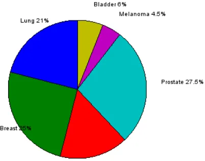
Scilab code Exa 2.2b pie chart

1 values = [42 50 32 55 9 12];

2 p e r c e n t a g e s = values *100 / sum( values ) ;

3 new_text = string( p e r c e n t a g e s ) ;

4 text = [” Lung ”, ” B r e a s t ”, ” Colon ”, ” P r o s t a t e ”, ” Melanoma ”, ” B l a d d e r ”];

(13)

(14)

7 // p i e ( [ 4 2 50 32 55 9 1 2 ] , [ ” Lung ” , ” B r e a s t ” , ” Colon ” , ” P r o s t a t e ” , ” Melanoma ” , ” B l a d d e r ” ] ) ;

8 pie ( values , f i n a l _ t e x t ) ;

Scilab code Exa 2.3a Sample mean

1 scores =[284 , 280 , 277 , 282 , 279 , 285 , 281 , 283 , 278 , 277];

2 n e w _ s c o r e s = scores - 280;

3 f i n a l _ m e a n = mean( n e w _ s c o r e s ) + 280;

4 disp( f i n a l _ m e a n )

Scilab code Exa 2.3b Sample mean of age

1 age = [15 16 17 18 19 20];

2 f r e q u e n c i e s = [2 5 11 9 14 13];

3 product = age .* f r e q u e n c i e s ;

4 t o t a l _ p e o p l e = sum( f r e q u e n c i e s ) ;

5 mean_age = sum( product ) / t o t a l _ p e o p l e ;

6 disp(” The s a m p l e mean o f t h e a g e s i s ”)

7 disp( mean_age )

Scilab code Exa 2.3c Sample Median

1 age = [15 16 17 18 19 20];

2 f r e q u e n c i e s = [2 5 11 9 14 13];

3 i =1;

4 for j =1:6

(15)

7 i = i +1 ;

Scilab code Exa 2.3d Mean and Median

1 g e r m _ f r e e _ m i c e = [158 192 193 194 195 202 212 215 229 230 237 240 244 247 259 301 301 321 337 415 434 444 485 496 529 537 624 707 800];

2 c o n v e n t i o n a l _ m i c e = [159 189 191 198 235 245 250 256 261 265 266 280 343 356 383 403 414 428 432];

3 disp (mean( g e r m _ f r e e _ m i c e ) , ” Sample mean f o r germ−

Scilab code Exa 2.3e Mean Median and Mode

(16)

8 end;

9 end

10 product = value .* f r e q u e n c i e s ;

11 disp( product , sum( product ) )

12

13 t o t a l _ v a l u e = sum( f r e q u e n c i e s ) ;

14 m e a n _ v a l u e = sum( product ) / t o t a l _ v a l u e ; // t h e a n s w e r i n t h e t e x t b o o k i s i n c o r r e c t

15 [ m1 m2 ]= max( f r e q u e n c i e s ) ;

16 n = m2 ;

17

18 disp(” The s a m p l e mean i s ”)

19 disp( m e a n _ v a l u e )

20 disp(median( f i n a l _ v a l u e ) , ” The median i s ”)

21 disp( value ( n ) , ” The mode i s ”)

Scilab code Exa 2.3f sample variance

1 A = [ 3 4 6 7 10];

2 B = [ -20 5 15 24];

3 disp(variance( A ) , ” The s a m p l e v a r i a n c e o f A i s ”)

4 disp(variance( B ) , ” The s a m p l e v a r i a n c e o f B i s ”)

Scilab code Exa 2.3g sample variance of accidents

1 a cc id e nt s = [22 22 26 28 27 25 30 29 24];

2 n e w _ a c c i d e n t s = ac c id en t s - 22;

(17)

Scilab code Exa 2.3h Percentile

1 p o p u l a t i o n = [7333253 3448613 2731743 1702086 1524249 1151977 1048949 1022830 998905 992038 816884 752279 734676 702979 665070 635913 617044 614289 579307 567094 547727 520947 514013 504505 493559];

2 disp(perctl( population , 10) , ” The s a m p l e 10 p e r c e n t i l e i s ”)

5 disp(median( p o p u l a t i o n ) , ” The median i s ”)

Scilab code Exa 2.3i Quartiles

1 noise = [ 82 89 94 110 74 122 112 95 100 78 65 60 90 83 87 75 114 85 69 94 124 115 107 88 97 74 72

68 83 91 90 102 77 125 108 65];

2 disp(quart( noise ) , ” The q u a r t i l e s a r e ”)

Scilab code Exa 2.4a Chebyshev Inequality

1 cars = [448162 404192 368327 318308 272122 260486 249128 234936 218540 207977];

2 i nt er v al 1 = mean( cars ) - (1.5*s t _ d e v i a t i o n( cars ) ) ;

3 i nt er v al 2 = mean( cars ) + (1.5*s t _ d e v i a t i o n( cars ) ) ;

4 data = 100*5/9;

(18)

Scilab code Exa 2.5a Empirical Rule

1 data = [90 91 94 83 85 85 87 88 72 74 74 75 77 77 78 60 62 63 64 66 66 52 55 55 56 58 43 46];

2 disp(” A c c o r d i n g t o t h e e m p i r i c a l r u l e ”)

3 disp(” 68% o f t h e d a t a l i e s b e t w e e n ”)

4 disp(mean( data ) +s t _ d e v i a t i o n( data ) , ” and ”, mean( data ) -s t _ d e v i a t i o n( data ) )

5 disp(” 95% o f t h e d a t a l i e s b e t w e e n ”)

6 disp(mean( data ) +(2*s t _ d e v i a t i o n( data ) ) , ” and ”, mean( data ) -(2*s t _ d e v i a t i o n( data ) ) )

7 disp(” 9 9 . 7% o f t h e d a t a l i e s b e t w e e n ”)

8 disp(mean( data ) +(3*s t _ d e v i a t i o n( data ) ) , ” and ”, mean( data ) -(3*s t _ d e v i a t i o n( data ) ) )

Scilab code Exa 2.6a Sample Correlation Coefficient

1 temp = [24.2 22.7 30.5 28.6 25.5 32.0 28.6 26.5 25.3 26.0 24.4 24.8 20.6 25.1 21.4 23.7 23.9 25.2 27.4 28.3 28.8 26.6];

2 defects = [25 31 36 33 19 24 27 25 16 14 22 23 20 25 25 23 27 30 33 32 35 24];

3 temp_new = temp - mean( temp ) ;

4 d e f e c t s _ n e w = defects - mean( defects ) ;

5 num =0

6 s1 =0;

7 s2 =0;

8 for i =1:22

9 num = num + ( temp_new ( i ) * d e f e c t s _ n e w ( i ) ) ;

10 s1 = s1 + ( temp_new ( i ) * temp_new ( i ) ) ;

(19)

13 c o e f f i c i e n t = num /sqrt( s1 * s2 ) ;

14 disp( c o e f f i c i e n t )

Scilab code Exa 2.6b Sample Correlation Coefficient

1 year = [12 16 13 18 19 12 18 19 12 14];

2 p ul se r at e = [73 67 74 63 73 84 60 62 76 71];

3 year_new = year - mean( year ) ;

4 p u l s e r a t e _ n e w = pu l se ra t e - mean( p u ls er a te ) ;

5 num =0

6 s1 =0;

7 s2 =0;

8 for i =1:10

9 num = num + ( year_new ( i ) * p u l s e r a t e _ n e w ( i ) ) ;

10 s1 = s1 + ( year_new ( i ) * year_new ( i ) ) ;

11 s2 = s2 + ( p u l s e r a t e _ n e w ( i ) * p u l s e r a t e _ n e w ( i ) ) ;

12 end

13 c o e f f i c i e n t = num /sqrt( s1 * s2 ) ;

(20)

Chapter 3 Elements Of Probability

Scilab code Exa 3.4a Union

1 c ig ar e tt e = 0.28;

2 cigar = 0.07;

3 c i g a r _ a n d _ c i g a r e t t e = 0.05 ;

4 c i g a r _ o r _ c i g a r e t t e = c i ga re t te + cigar -c i g a r _ a n d _ -c i g a r e t t e ;

5 disp( ”% o f t h e m a l e s smoke n e i t h e r c i g a r n o r c i g a r e t t e ”, (1 - c i g a r _ o r _ c i g a r e t t e ) *100 )

Scilab code Exa 3.5a Basic Principle of Counting

1 w h i t e _ b a l l s = 6;

2 b l a c k _ b a l l s = 5;

3 total = w h i t e _ b a l l s + b l a c k _ b a l l s ;

4 p r o b a b i l i t y _ w h i t e a n d b l a c k = w h i t e _ b a l l s * b l a c k _ b a l l s /( total *( total -1) ) ;

5 p r o b a b i l i t y _ b l a c k a n d w h i t e = w h i t e _ b a l l s * b l a c k _ b a l l s /( total *( total -1) ) ;

(21)

7 disp( reqd_probability , ” Thus , t h e r e q u i r e d p r o b a b i l i t y i s ”)

Scilab code Exa 3.5b Basic Principle of Counting

1 maths = 4;

2 c he mi s tr y = 3;

3 history = 2;

4 language = 1;

5 t o t a l _ a r r a n g e m e n t s = f a ct or i al (4) * f ac t or ia l ( maths ) * f ac to r ia l ( c he mi s tr y ) * f ac to r ia l ( history ) * f ac t or ia l ( language ) ;

6 disp( to t al _a r ra n ge me n ts , ” The t o t a l number o f p o s s i b l e a r r a n g e m e n t s i s ”)

Scilab code Exa 3.5c Basic Principle of Counting

1 men = 6;

2 women = 4;

3 disp( fa c to ri a l ( men + women ) , ”No o f d i f f e r e n t r a n k i n g s p o s s i b l e i s ”)

4 w o m e n _ t o p 4 = f ac to r ia l ( women ) * f a ct or i al ( men ) ;

5 prob = w o m e n _ t o p 4 / fa c to ri a l ( men + women ) ;

6 disp( prob , ” P r o b a b i l i t y t h a t women r e c e i v e t h e t o p 4 s c o r e s i s ”)

Scilab code Exa 3.5d Committee Probability

1 men = 6;

(22)

3 r eq d_ s iz e =5;

4 total_p = black_p + white_p ;

(23)

20 black_p = black_p -2;

21 // d i s p ( b l a c k p a i r s )

22 end

23 b l a c k _ p a i r s = b l a c k _ p a i r s / fa ct o ri al (3) ;

24 // d i s p ( b l a c k p a i r s )

25 26

27 w h i t e _ p a i r s = b l a c k _ p a i r s ;

28 a l l o w e d _ p a i r s = b l a c k _ p a i r s * w h i t e _ p a i r s ;

29 probb = a l l o w e d _ p a i r s / t o t a l _ p a i r s ;

30 disp( probb , ” P r o b a b i l i t y t h a t a random p a i r i n g w i l l n o t r e s u l t i n any o f t h e w h i t e and b l a c k p l a y e r s r o o m i n g t o g e t h e r i s ”)

Scilab code Exa 3.6a Acceptable Transistor

1 d ef ec t iv e =5;

2 p a r t i a l l y _ d e f e c t i v e = 10;

3 a c c e p t a b l e = 25;

4 disp( a c c e p t a b l e /( a c c e p t a b l e + p a r t i a l l y _ d e f e c t i v e ) , ” The r e q u i r e d p r o b a b i l i t y i s ”)

Scilab code Exa 3.6b Both Boys

1 prob_bb = 0.25;

2 prob_bg = 0.25;

3 prob_gb = 0.25;

4 prob_gg = 0.25;

(24)

Scilab code Exa 3.6c Branch Manager

1 p r o b _ p h o e n i x = 0.3;

2 p r o b _ m a n a g e r = 0.6;

3 disp( p r o b _ p h o e n i x * p r o b _ m a n a g e r , ” P r o b a b i l i t y t h a t P e r e z w i l l be a P h o e n i x b r a n c h o f f i c e manager i s ”

)

Scilab code Exa 3.7a Accident Probability

1 a c c i d e n t _ p r o n e = 0.4;

2 n o n a c c i d e n t _ p r o n e = 0.2;

3 p o p _ a c c i d e n t = 0.3;

4 prob = p o p _ a c c i d e n t * a c c i d e n t _ p r o n e + (1 - p o p _ a c c i d e n t ) * n o n a c c i d e n t _ p r o n e ;

5 disp( prob , ” The r e q u i r e d p r o b a b i l i t y i s ”) ;

Scilab code Exa 3.7b Accident within a year

1 a c c i d e n t _ p r o n e = 0.4;

2 n o n a c c i d e n t _ p r o n e = 0.2;

3 p o p _ a c c i d e n t = 0.3;

4 p r o b _ o f _ a c c i d e n t = p o p _ a c c i d e n t * a c c i d e n t _ p r o n e + (1 -p o -p _ a c c i d e n t ) * n o n a c c i d e n t _ -p r o n e ;

5 prob = p o p _ a c c i d e n t * a c c i d e n t _ p r o n e / p r o b _ o f _ a c c i d e n t ;

6 disp( prob , ” The r e q u i r e d p r o b a b i l i t y i s ”)

(25)

1 m = 5;

2 p =1/2;

3 disp( ( m * p ) /(1+(( m -1) * p ) ) , ” The r e q u i r e d p r o b a b i l i t y i s ”)

Scilab code Exa 3.7d blood test

1 d e t e c t _ p r e s e n t = 0.99;

2 d e t e c t _ n o t p r e s e n t = 0.01;

3 p o p _ d i s e a s e = 0.005;

4 prob = d e t e c t _ p r e s e n t * p o p _ d i s e a s e /(( d e t e c t _ p r e s e n t * p o p _ d i s e a s e ) +( d e t e c t _ n o t p r e s e n t *(1 - p o p _ d i s e a s e ) )

) ;

Scilab code Exa 3.7e Criminal Investigation

1 c r i m i n a l _ c h a r = 0.9

2 c on vi n ce d = 0.6;

3 pop_char = 0.2;

4 prob = ( co n vi nc e d * c r i m i n a l _ c h a r ) /(( co nv i nc e d * c r i m i n a l _ c h a r ) + ( pop_char *(1 - c o nv in c ed ) ) ) ;

Scilab code Exa 3.7f Missing Plane

1 alpha1 = 0.4;

2 p l a n e _ i n _ r e g i o n 1 = 1/3;

3 p l a n e _ i n _ r e g i o n 2 = 1/3;

(26)

5 prob1 = ( alpha1 * p l a n e _ i n _ r e g i o n 1 ) /(( alpha1 * p l a n e _ i n _ r e g i o n 1 ) + 1* p l a n e _ i n _ r e g i o n 2 + 1* p l a n e _ i n _ r e g i o n 3 ) ;

6 prob2 = (1* p l a n e _ i n _ r e g i o n 2 ) /(( alpha1 *

p l a n e _ i n _ r e g i o n 1 ) + 1* p l a n e _ i n _ r e g i o n 2 + 1* p l a n e _ i n _ r e g i o n 3 ) ;

7 disp( prob1 , ” The p r o b a b i l i t y t h a t t h e p l a n e s i s i n r e g i o n 1 g i v e n t h a t t h e s e a r c h o f r e g i o n 1 d i d n o t u n c o v e r i t ”) ;

8 disp( prob2 , ” The p r o b a b i l i t y t h a t t h e p l a n e s i s i n r e g i o n 2/3 g i v e n t h a t t h e s e a r c h o f r e g i o n 1 d i d n o t u n c o v e r i t ”) ;

Scilab code Exa 3.8a Independent Events

1 prob_A = 4/52;

2 prob_H = 13/52;

(27)

Chapter 4 Random Variables And

Expectation

Scilab code Exa 4.1a sum of two fair dice

1 p11 = 1/36;

2 p12 = 1/36;

3 p13 = 1/36;

4 p14 = 1/36;

5 p15 = 1/36;

6 p16 = 1/36;

7 p21 = 1/36;

8 p22 = 1/36;

9 p23 = 1/36;

10 p24 = 1/36;

11 p25 = 1/36;

12 p26 = 1/36;

13 p31 = 1/36;

14 p32 = 1/36;

15 p33 = 1/36;

16 p34 = 1/36;

17 p35 = 1/36;

18 p36 = 1/36;

(28)

(29)

1 pdd = 0.09;

2 pda = 0.21;

3 pad = 0.21;

4 paa = 0.49;

5

6 disp( pdd , ” P r o b a b i l i t y t h a t t h e number o f a c c e p t a b l e c o m p o n e n ts i s 0 i s ”)

7 disp( pda + pad , ” P r o b a b i l i t y t h a t t h e number o f a c c e p t a b l e c o m p o ne n t s i s 1 i s ”)

8 disp( paa , ” P r o b a b i l i t y t h a t t h e number o f a c c e p t a b l e c o m p o n e n ts i s 2 i s ”)

9 disp( pdd , ” P r o b a b i l i t y t h a t I i s 0 i s ”)

10

11 disp( paa + pad + pda , ” P r o b a b i l i t y t h a t I i s 1 i s ”)

Scilab code Exa 4.1c X exceeds 1

1 prob = 1 -(1 -(1/ %e ) ) ;

2 disp( prob , ” P r o b a b i l i t y t h a t X e x c e e d s 1 i s ”)

Scilab code Exa 4.2a sum of pmf

1 p1 = 1/2;

2 p2 = 1/3;

3 disp (1 -( p1 + p2 ) , ” P r o b a b i l i t y t h a t X i s 3 i s ”)

Scilab code Exa 4.2b pdf

1

(30)

3 C = 1/ integral ;

Scilab code Exa 4.3a Joint distribution of batteries

(31)

13 disp( fa c to ri a l (3) * fa ct o ri al (4) /( f ac t or i al (2) * f ac to r ia l (1) * fa c to ri a l (3) * total ) , ” P r o b a b i l i t y t h a t X=2 and Y=1”) ;

14 disp( fa c to ri a l (3) /( f a ct o ri al (3) * total ) , ” P r o b a b i l i t y t h a t X=3 and Y=3”) ;

Scilab code Exa 4.3b Joint distribution of boys and girls

(32)

Scilab code Exa 4.3c Joint Density Function

1 intx = i n te gr a te( ’ %eˆ(−x ) ’, ’ x ’,0 , 1 ) ;

2 inty =in t eg ra t e( ’ 2∗%eˆ(−2∗y ) ’, ’ y ’, 0 , 1) ;

3 answer = (1 - intx ) * inty ;

4 disp( answer , ” P r o b a b i l i t y t h a t X>1 and Y<1 i s ”) 5

6 // For o t h e r two p a r t s , s y m b o l i c m a n i p u l a t i o n s a r e r e q u i r e d

Scilab code Exa 4.3e Density of Independent Random Variables

1 pdec3 = 0.05;

2 pdec2 = 0.1;

3 pdec1 = 0.2;

4 p0 = 0.3

5 pinc1 = 0.2;

6 pinc2 = 0.1;

7 pinc3 = 0.05;

8 disp( pinc1 * pinc2 * p0 , ” P r o b a b i l i t y t h a t t h e s t o c k p r i c e w i l l i n c r e a s e s u c c e s s i v e l y by 1 , 2 and 0 p o i n t s i n t h e n e x t 3 d a y s i s ”)

Scilab code Exa 4.3f Conditional Probability Mass Function

1 disp(0.1/0.3875 , ” p r o b a b i l i t y t h a t B =0 g i v e n G=1 ”) ;

(33)

Scilab code Exa 4.3g Conditional Probability Mass Function

1 p00 =0.4;

2 p01 = 0.2;

3 p10 = 0.1;

4 p11 = 0.3;

5

6 pY1 = p01 + p11 ;

7 disp( p01 / pY1 , ” P r o b a b i l i t y t h a t X=0 and Y=1”)

8 disp( p11 / pY1 , ” P r o b a b i l i t y t h a t X=1 and Y=1”)

Scilab code Exa 4.4a Expectation of a fair die

1 p1 =1/6;

2 p2 =1/6;

3 p3 =1/6;

4 p4 =1/6;

5 p5 =1/6;

6 p6 =1/6;

7 expec = p1 + (2* p2 ) +(3* p3 ) +(4* p4 ) +(5* p5 ) + (6* p6 ) ;

8 disp( expec )

Scilab code Exa 4.4d Expectation of the message time

1 expec = in t eg ra t e( ’ ( x ) / 1 . 5 ’, ’ x ’, 0 ,1.5) ;

(34)

Scilab code Exa 4.5a Expectation

1 p0 = 0.2;

2 p1 = 0.5;

3 p2 =0.3;

4 expec = 0*0* p0 + 1*1* p1 + 2*2* p2 ;

5 disp( expec , ” E x p e c t a t i o n o f Xˆ2 i s ”)

Scilab code Exa 4.5b Expected cost of breakdown

1 expec = i nt e gr a te( ’ x ˆ3 ’, ’ x ’, 0 , 1) ;

2 disp( expec , ” The e x p e c t a t i o n i s ”)

Scilab code Exa 4.5c Expectation

1 p0 = 0.2;

2 p1 = 0.5;

3 p2 =0.3;

4 expec = 0*0* p0 + 1*1* p1 + 2*2* p2 ;

5 disp( expec , ” E x p e c t a t i o n o f Xˆ2 i s ”)

Scilab code Exa 4.5d Expectation

1 expec = i nt e gr a te( ’ x ˆ3 ’, ’ x ’, 0 , 1) ;

(35)

Scilab code Exa 4.5e Expected profit

1 profit1 = 10;

2 profit2 = 20;

3 profit3 = 40;

4 prob1 = 0.2;

5 prob2 = 0.8;

6 prob3 = 0.3;

7 expec = profit1 * prob1 + profit2 * prob2 + profit3 * prob3 ;

8 disp(” t h o u s a n d d o l l a r s ”, expec , ” The e x p e c t d p r o f i t i s ”)

Scilab code Exa 4.5f Letters in Correct Envelopes

1 // As s c i l a b d o e s n o t s y m b o l i c c o m p u t a t i o n s , t h i s e x a m p l e i s s o l v e d t a k i n g N=5

2 prob = 1/5 // p r o b a b i l i t y t h a t a l e t t e r i s put i n t o t h e r i g h t e n v e l o p e

3 EX1 = 1* prob +0*(1 - prob ) ;

4 EX2 = 1* prob +0*(1 - prob ) ;

5 EX3 = 1* prob +0*(1 - prob ) ;

6 EX4 = 1* prob +0*(1 - prob ) ;

7 EX5 = 1* prob +0*(1 - prob ) ;

8 EX = EX1 + EX2 + EX3 + EX4 + EX5 ;

9 disp( EX , ” Thus , t h e e x p e c t a t i o n i s ”)

(36)

1 P r o b X i e q u a l s 1 = 1 - ((19/20) ^10) ;

2 EXi = P r o b X i e q u a l s 1 ;

3 EX = 20* EXi ;

4 disp( EX , ” The e x p e c t a t i o n i s ”)

Scilab code Exa 4.6a Variance of a fair die

1 p r o b X e q u a l s i = 1/6;

2 e x p e c X s q u a r e d = 0;

3 for n =1:6

4 e x p e c X s q u a r e d = e x p e c X s q u a r e d + ( n * n * p r o b X e q u a l s i )

5 end 6

7 expecX = 3.5 // from e g 4 . 4 a

8 var = e x p e c X s q u a r e d - ( expecX ^2) ;

9 disp( var , ” The v a r i a n c e i s ”)

Scilab code Exa 4.7a Variance of 10 rolls of a fair die

1 p r o b X e q u a l s i = 1/6;

2 e x p e c X s q u a r e d = 0;

3 for n =1:6

4 e x p e c X s q u a r e d = e x p e c X s q u a r e d + ( n * n * p r o b X e q u a l s i )

5 end 6

7 expecX = 3.5 // from e g 4 . 4 a

8 var = e x p e c X s q u a r e d - ( expecX ^2) ;

9 var10 = var *10;

(37)

Scilab code Exa 4.7b Variance of 10 tosses of a coin

1 probIj = 0.5;

2 varIj = probIj *(1 - probIj ) ;

3 var = 10* varIj ;

4 disp( var , ” Thus , t h e r e q u i r e d v a r i a n c e i s ”)

Scilab code Exa 4.9a Inequalities

1 avg = 50;

2 probX75 = avg /75;

3 disp( probX75 , ” P r o b a b i l i t y t h a t X>75 i s ”) 4 var = 25;

5 u p p e r l i m i t = var /100;

(38)

Chapter 5 Special Random Variables

Scilab code Exa 5.1a Returning of disks

1 defects = 0.01;

2 disks = 10;

3 package = 3;

4 p r o b d e f e c t 0 = ((1 - defects ) ^10) ;

5 p r o b d e f e c t 1 = f ac t or ia l ( disks ) * defects *((1 - defects ) ^9) / f ac t or ia l ( disks -1) ;

6 prob = 1 - p r o b d e f e c t 0 - p r o b d e f e c t 1 ;

7 disp( prob , ” P r o b a b i l i t y t h a t a p a c k a g e w i l l be r e t u r n e d i s ”)

8 newprob = fa c to ri a l ( package ) * prob *((1 - prob ) ^2) / f ac to r ia l ( package -1) ;

9 disp( newprob , ” P r o b a b i l i t y t h a t e x a c t l y one o f t h e p a c k a g e s w i l l be r e t u r n e d among 3 i s ” )

10

11 // t h e s o l u t i o n i n t h e t e x t b o o k i s a p p r o x i m a t e

(39)

1 function result = binomial(n , k , p )

Scilab code Exa 5.1e Binomial Random Variable

1 function result = bin (n ,k , p )

(40)

1 [ probX0 , Q ]= cdfpoi(”PQ”, 0 , 3) ;

2 probX1 = 1 - probX0 ;

3 disp( probX1 , ” P r o b a b i l i t y t h a t t h e r e i s a t l e a s t one a c c i d e n t t h i s week i s ”)

Scilab code Exa 5.2b Defective Items

1 function result = bino (n , k , p )

2 result = fa c to ri a l ( n ) *( p ^ k ) *((1 - p ) ^( n - k ) ) /( f ac to r ia l ( k ) * fa c to ri a l (n - k ) )

3 e n d f u n c t i o n 4

5 prob = bino (10 ,0 , 0.1) + bino (10 , 1 ,0.1 ) ;

6 disp( prob , ” The e x a c t p r o b a b i l i t y i s ”) ;

7

8 probp = cdfpoi(”PQ”, 1 , 1)

9 disp( probp , ” The p o i s s o n a p p r o x i m a t i o n i s ”)

Scilab code Exa 5.2c Number of Alpha particles

1 Xlam = 3.2;

2 i =2;

3 prob = cdfpoi(”PQ”, i , Xlam ) ;

4 disp( prob )

Scilab code Exa 5.2d Claims handled by an insurance company

(41)

3 e n d f u n c t i o n 4 avg = 5;

5 i =3;

6 prob = cdfpoi(”PQ”, 2 , avg ) ;

7 disp( prob , ” P r o p o r t i o n o f d a y s t h a t have l e s s t h a n 3 c l a i m s i s ”)

8 probX4 = cdfpoi(”PQ”,i +1 , avg ) - cdfpoi(”PQ”, i , avg ) ;

9

10 reqdprob = bino (5 ,3 , probX4 ) ;

11 disp( reqdprob , ” P r o b a b i l i t y t h a t 3 o f t h e n e x t 5 d a y s w i l l have e x a c t l y 4 c l a i m s i s ”)

Scilab code Exa 5.2f Defective stereos

1 avg = 4;

2 prob = cdfpoi(”PQ”, 3 , 2* avg )

3 disp( prob )

Scilab code Exa 5.3a Functional system

1 function result = hyper (N , M , n , i )

2 result = fa c to ri a l ( N ) * fa ct o ri al ( M ) * f a ct or i al ( n ) * f ac to r ia l ( N +M - n ) /( f a ct or i al ( i ) * f ac t or ia l (N - i ) * f ac t or ia l (n - i ) * fa c to ri a l (M - n + i ) * f ac t or ia l ( N + M ) ) ;

5 prob = hyper (15 , 5 ,6 , 4) + hyper (15 , 5 ,6 ,5) + hyper (15 ,5 ,6 ,6) ;

(42)

Scilab code Exa 5.3b Determining Population Size

1 function result = hyper (N , M , n , i )

2 result = fa c to ri a l ( N ) * fa ct o ri al ( M ) * f a ct or i al ( n ) * f ac to r ia l ( N +M - n ) /( f a ct or i al ( i ) * f ac t or ia l (N - i ) * f ac t or ia l (n - i ) * fa c to ri a l (M - n + i ) * f ac t or ia l ( N + M ) ) ;

5 r = 50;

6 n =100;

7 X =25;

8 disp( r * n / X , ” E s t i m a t e o f t h e number o f a n i m a l s i n t h e r e g i o n i s ”)

Scilab code Exa 5.3c Conditional Probability

5 function answer = condprob (n ,k ,p , i )

6 answer = bino (n ,i , p ) * bino (m ,k -i , p ) / bino ( n +m ,k , p ) ;

(43)

Scilab code Exa 5.4b Bus Timings

1 pass_f = 1/30;

2 prob1 = (15 -10) * pass_f + (30 -25) * pass_f ;

3 prob2 = (3 -0) * pass_f + (18 -15) * pass_f ;

4 disp( prob1 , ” P r o b a b i l i t y t h a t he w a i t s l e s s t h a n 5 m i n u t e s f o r a bus ”)

5 disp( prob2 , ” P r o b a b i l i t y t h a t he w a i t s a t l e a s t 12 m i n u t e s f o r a bus ”)

Scilab code Exa 5.4c Current in a diode

1 a =5;

2 I0 =10^ -6;

3 v_f = 1/(3 -1) ;

4 v up pe r li m = 3;

5 v lo we r li m = 1;

6 expecV = ( vu pp e rl i m + vl o we rl i m ) /2;

7 expec = i nt e gr a te( ’ ( %e ˆ ( a∗x ) ) /2 ’, ’ x ’, 1 ,3) ;

8 expecI = I0 *( expec -1) ;

9 disp( expecI )

Scilab code Exa 5.5a Normal Random Variable

1 u = 3;

2 var = 16;

3

4 prob1 = cdfnor(”PQ”, 11 , u , sqrt( var ) ) ;

5 disp( prob1 , ” P{X<11}”) ;

6 prob2 = 1 - cdfnor( ”PQ”, -1 , u , sqrt( var ) ) ;

7 disp( prob2 , ”P{X>−1}”) ;

(44)

9 disp( prob3 , ”P{2<X<7}”) ;

Scilab code Exa 5.5b Noise in Binary Message

1 disp(cdfnor(”PQ”, -1.5 , 0 , 1) , ”P{e r r o r |m e s s a g e i s 1}”)

2 disp(1 -cdfnor(”PQ”, 2.5 , 0 , 1) , ”P{e r r o r |m e s s a g e i s 0 }”)

Scilab code Exa 5.5c Power dissipation

1 r =3;

2 avg = 6;

3 std = 1;

4 var = std ^2;

5 expecV2 = var + ( avg ^2) ;

6 expecW = 3* expecV2 ;

7 disp( expecW , ” E x p e c t a t i o n o f W i s ”)

8 limw =120;

9 limV = sqrt( limw / r ) ;

10 disp(1 -cdfnor(”PQ”, limV , avg , std ) , ”P{W>120} i s ”)

Scilab code Exa 5.5d Yearly precipitation

1 meanX1 = 12.08;

2 meanX2 = 12.08;

3 stX1 = 3.1;

4 meanX = meanX1 + meanX2 ;

(45)

7 disp(1 -cdfnor(”PQ”, lim , meanX , sqrt( varX ) ) , ” P r o b a b i l i t y t h a t t h e t o t a l p r e c i p i t a t i o n d u r i n g t h e n e x t 2 y e a r s w i l l e x c e e d 25 i n c h e s ”)

8

9 meanXnew = meanX1 - meanX2 ;

10 new_lim = 3;

11 disp(1 - cdfnor(”PQ”, new_lim , meanXnew , sqrt( varX ) ) ,

” P r o b a b i l i t y t h a t p r e c i p i t a t i o n i n t h e n e x t y e a r w i l l e x c e e d t h a t i n t h e f o l l o w i n g y e a r by more t h a n 3 i n c h e s ”)

Scilab code Exa 5.6a Wearing of Battery

1 lamda = 1/10000;

2 x = 5000;

3 prob = %e ^( -1* lamda * x ) ;

4 disp( prob , ” P r o b a b i l i t y t h a t s h e w i l l be a b l e t o c o m p l e t e h e r t r i p w i t h o u t h a v i n g t o r e p l a c e h e r c a r b a t t e r y i s ”) ;

Scilab code Exa 5.6b Working Machines

1 //When C i s put t o use , one o t h e r machine ( e i t h e r A o r B ) w i l l s t i l l be w o r k i n g . The p r o b a b i l i t y o f

t h i s machine o r C f a i l i n g i s e q u a l due t o t h e m e m o r y l e s s p r o p o e r t y o f e x p o n e n t i a l random v a r i a b l e s .

2

(46)

Scilab code Exa 5.6c Series System

1 function result = new ( lamda ,n , t )

2 newsum = 0;

3 for i =1: n

4 newsum = newsum + lamda ( i )

5 result = %e ^( -1* newsum * t )

6 end

7 e n d f u n c t i o n

Scilab code Exa 5.8a Chi square random variable

1 disp(cdfchn(”PQ”, 30 , 26 , 0) ) ;

Scilab code Exa 5.8b Chi square random variable

1 disp(cdfchn(”X”, 15 , 0 ,0.95 , 0.05 ) )

Scilab code Exa 5.8c Locating a Target

1 disp(1 - cdfchn(”PQ”, 9/4 , 3 , 0) )

Scilab code Exa 5.8d Locating a Target in 2D space

(47)

Scilab code Exa 5.8e T distribution

1 disp(cdft(”PQ”, 1.4 , 12) , ”P{T12 <=1.4}”) ; 2 disp(cdft(”T”, 9 , 0.975 , 0.025) , ” t 0 . 0 2 5 , 9 ”)

Scilab code Exa 5.8f F Distribution

(48)

Chapter 6 Distribution of Sampling

Statistics

Scilab code Exa 6.3a Claims handled by an insurance company

1 number = 25000;

2 meaneach = 320;

3 sdeach = 540;

4 claim = 8300000;

5 m ea nt o ta l = meaneach * number ;

6 sdtotal = sdeach *sqrt( number ) ;

7 disp(1 - cdfnor(”PQ”, claim , meantotal , sdtotal ) )

Scilab code Exa 6.3c Class strength

1 i de al _ nu m = 150;

2 a c t u a l _ n u m = 450;

3 attend = 0.3;

4 t ol er a nc e = 0.5

(49)

Scilab code Exa 6.3d Weights of workers

1 meaneach = 167;

2 sdeach = 27;

3 num = 36;

4 sdtotal = sdeach /sqrt( num ) ;

5 // s d t o t a l = s d t o t a l∗s d t o t a l ;

6 // d i s p ( s d t o t a l )

7 disp(cdfnor(”PQ”, 170 , meaneach , sdtotal ) -cdfnor(”PQ ”, 163 , meaneach , sdtotal ) , ” P r o b a b i l i t y t h a t t h e

s a m p l e mean o f t h e i r w e i g h t s l i e s b e t w e e n 163 and 1 7 0 ( when s a m p l e s i z e i s 3 6 ) ”)

8

9 num =144;

10 sdtotal = sdeach /sqrt( num ) ;

11 // d i s p ( s d t o t a l )

12 disp(cdfnor(”PQ”, 170 , meaneach , sdtotal ) -cdfnor(”PQ ”, 163 , meaneach , sdtotal ) , ” P r o b a b i l i t y t h a t t h e

s a m p l e mean o f t h e i r w e i g h t s l i e s b e t w e e n 163 and 1 7 0 ( when s a m p l e s i z e i s 1 4 4 ) ”)

13

14 // The a n s w e r g i v e n i n t h e t e x t b o o k i s i n c o r r e c t a s (170−167) / 4 . 5 i s n o t e q u a l t o 0 . 6 2 5 9 .

Scilab code Exa 6.3e Distance of a start

1 prob = 0.95;

2 lim = 0.5;

3 X = cdfnor(”X”, 0 ,1 , 0.975 , 0.025 )

(50)

Scilab code Exa 6.5a Processing time

1 n = 15;

2 s i g m a s q u a r e = 9;

3 lim =12;

4 a c t u a l _ l i m = (n -1) * lim / s i g m a s q u a r e ;

5 prob = 1 - cdfchi(”PQ”, actual_lim , (n -1) )

6 disp( prob )

Scilab code Exa 6.6a Candidate winning an election

1 favour = 0.45;

2 s a m p l e s i z e = 200;

3 expec = favour * s a m p l e s i z e ;

4 sd = sqrt( s a m p l e s i z e * favour *(1 - favour ) ) ;

5 disp( expec , ” The e x p e c t e d v a l u e i s ”)

6 disp( sd , ” The s t a n d a r d d e v i a t i o n i s ”)

7

12 // newsum = 0 ;

13 // f o r i =1:10

14 // newsum = newsum + b i n o ( 2 0 0 , i , f a v o u r )

15 // end

16 // p r o b = 1−newsum ;∗/

17

18 lim = 101;

(51)

21 prob = 1 - cdfnor(”PQ”, lim , expec , sd )

22

23 disp( prob , ” P r o b a b i l i t y t h a t more t h a n h a l f t h e members o f t h e s a m p l e f a v o u r t h e c a n d i d a t e ”)

Scilab code Exa 6.6b Pork consumption

1 meaneach = 147;

2 sdeach = 62;

3 s a m p l e s i z e = 25;

4 lim =150;

5 s a m p l e m e a n = meaneach ;

6 samplesd = sdeach /sqrt( s a m p l e s i z e )

7 prob = 1 - cdfnor(”PQ”, lim , samplemean , samplesd )

(52)

Chapter 7 Parameter Estimation

Scilab code Exa 7.2a Maximum likelihood estimator of a bernoulli pa-rameter

1 s a m p l e s i z e = 1000;

2 a c c e p t a b l e =921;

3 disp( a c c e p t a b l e / samplesize , ” The maximum l i k e l i h o o d e s t i m a t e o f p i s ”)

Scilab code Exa 7.2b Errors in a manuscript

1 function result = t o t a l e r r o r ( n1 , n2 , n12 )

2 result = n1 * n2 / n12 ;

(53)

2 days = 20;

3 disp( t o t a l _ p e o p l e / days , ” The maximum l i k e l i h o o d e s t i m a t e o f lambda ”)

Scilab code Exa 7.2d Number of traffic accidents

1 a cc id e nt s = [4 0 6 5 2 1 2 0 4 3 ];

2 lambda = mean( ac c id en t s )

3 disp(cdfpoi(”PQ”, 2 , lambda ) )

Scilab code Exa 7.2e Maximum likelihood estimator in a normal popula-tion

1 function[u , s i g m a s q u a r e d ]= normal (X , Xmean , n )

2 u = Xmean ;

3 newsum = 0;

4 for i = 1: n

5 newsum = newsum + ( X ( i ) - Xmean ) ^2

6 end

7 s i g m a s q u a r e d = sqrt(( newsum / n ) ) ;

Scilab code Exa 7.2f Kolmogorovs law of fragmentation

1 X = [2.2 3.4 1.6 0.8 2.7 3.3 1.6 2.8 2.5 1.9]

2 u pp er l im X = 3

3 l ow er l im X = 2;

4 u p p e r l i m l o g X = log( up pe r li mX ) ;

5 l o w e r l i m l o g X = log( l ow er l im X ) ;

(54)

7 logX = log( X )

8 s a m p l e m e a n = mean( logX )

9 samplesd = sqrt(variance( logX ) )

10 // d i s p ( samplemean )

11 // d i s p ( s a m p l e s d )

12 prob = cdfnor(”PQ”, upperlimlogX , samplemean ,

samplesd ) - cdfnor(”PQ”, lowerlimlogX , samplemean , samplesd )

13 disp( prob )

Scilab code Exa 7.2g Estimating Mean of a Uniform Distribution

1 function result = unif (X , n )

2 result = max( X ) /2;

Scilab code Exa 7.3a Error in a signal

1 avg = 0;

2 var = 4;

3 num = 9;

4 X =[5 8.5 12 15 7 9 7.5 6.5 10.5];

5 s a m p l e m e a n = mean( X ) ;

6 lowerlim = s a m p l e m e a n - (1.96*sqrt( var / num ) )

7 upperlim = s a m p l e m e a n + (1.96*sqrt( var / num ) )

8

(55)

(56)

Scilab code Exa 7.3d Weight of a salmon

1 sd = 0.3;

2 lim = 0.1;

3 num = (1.96* sd / lim ) ^2;

4 disp( num , ” Sample s i z e s h o u l d be g r e a t e r t h a n ”) ;

Scilab code Exa 7.3e Error in a signal

1 X = [5 8.5 12 15 7 9 7.5 6.5 10.5];

2 num = 9;

3 meanX = mean( X ) ;

4 X2 = X ^2;

5 s2 = (sum( X2 ) - ( num *( meanX ^2) ) ) /( num -1) ;

6 s = sqrt( s2 ) ;

7 tval = cdft(”T”, num -1 , 0.975 , 0.025) ;

8 // d i s p ( t v a l )

9 upperlim = meanX + ( tval * s ) /sqrt( num ) ;

10 lowerlim = meanX - ( tval * s ) /sqrt( num ) ;

11 disp( upperlim , ” t o ”, lowerlim ,” The 95% c o n f i d e n c e i n t e r v a l i s ”, )

Scilab code Exa 7.3f Average resting pulse

1 X = [54 63 58 72 49 92 70 73 69 104 48 66 80 64 77];

2 num = 15;

(57)

6 s = sqrt( s2 ) ;

Scilab code Exa 7.3h Thickness of washers

1 num =10;

2 X = [0.123 0.133 0.124 0.126 0.120 0.130 0.125 0.128 0.124 0.126];

3 // d i s p ( v a r i a n c e (X) )

4 s2 = variance( X ) ;

(58)

(59)

(60)

Scilab code Exa 7.5a Transistors

1 phat = 0.8;

2 zalpha = 1.96;

3

4 s a m p l e s i z e = 100;

5 lowerlim = phat - ( zalpha *sqrt( phat *(1 - phat ) / s a m p l e s i z e ) ) ;

6 upperlim = phat + ( zalpha *sqrt( phat *(1 - phat ) / s a m p l e s i z e ) ) ;

7 disp( upperlim , ” t o ”, lowerlim ,” The 95% c o n f i d e n c e i n t e r v a l i s ” )

Scilab code Exa 7.5b Survey

1 phat = 0.52;

2 error = 0.04;

3 zalpha = 1.96;

4 // l o w e r l i m = p h a t − ( z a l p h a∗s q r t ( p h a t∗(1−p h a t ) / s a m p l e s i z e ) ) ;

5 // u p p e r l i m = p h a t + ( z a l p h a∗s q r t ( p h a t∗(1−p h a t ) / s a m p l e s i z e ) ) ;

6 s a m p l e s i z e = (error/ zalpha ) ^2/( phat *(1 - phat ) ) ;

7 disp(1/ s a m p l e s i z e )

Scilab code Exa 7.5c Acceptable chips

1 i n i t i a l s a m p l e = 30;

2 a c c e p t a b l e = 26;

3 phat = a c c e p t a b l e / i n i t i a l s a m p l e ;

4 error = 0.05/2;

(61)

7 s a m p l e s i z e = (error/ zalpha ) ^2/( phat *(1 - phat ) ) ;

Scilab code Exa 7.6a Life of a product

1 s um _l i ve s = 1740; chi -square(0.975 , 20) . The textbook says the value is

13 9.661 whereas scilab c a l c u l a t e s its value as 9.59

(62)

1 function result1 = e s t i m a t o r 1 ( X )

2 result1 = X (1) ;

3 // r e s u l t 2 = mean (X) ;

4

6 function result2 = e s t i m a t o r 2 ( X )

7 // r e s u l t 1 = X( 1 ) ;

8 result2 = mean( X ) ;

9

Scilab code Exa 7.7b Point estimator

1 function result1 = estimate (d , sigma )

2 sigmainv = 1/ sigma ;

3 new = d ./ sigma ;

4 result1 = sum( new ) /sum( sigmainv ) ;

7 function result2 = mserror ( sigma )

8 sigmainv = 1/ sigma ;

9

10 result1 = 1/sum( sigmainv ) ;

Scilab code Exa 7.7c Point estimator of a uniform distribution

1 function result = u n b i a s e d e s t i m a t o r (X , n )

2 c =( n +2) /( n +1) ;

3 result = c *max( X ) ;

(63)

Scilab code Exa 7.8a Bayes estimator

1 function result = es t im at o r (X , n )

2 result = (sum( X ) +1) /( n +2) ;

Scilab code Exa 7.8b Bayes estimator of a normal population

1 function result = m e a n e s t i m a t o r ( sigma0 , u , sigma , n , X )

3 result = ( n * meanX / sigma0 ) /(( n / sigma0 ) +(1/ sigma ) ) + ( u / sigma ) /(( n / sigma0 ) +(1/ sigma ) ) ;

6 function result = v a r e s t i m a t o r ( sigma0 , sigma , n )

7 result = ( sigma0 * sigma ) /(( n * sigma ) + sigma0 ) ;

Scilab code Exa 7.8d estimator of the signal value

1 function result = m e a n e s t i m a t o r ( sigma0 , u , sigma , n , X )

3 result = ( n * meanX / sigma0 ) /(( n / sigma0 ) +(1/ sigma ) ) + ( u / sigma ) /(( n / sigma0 ) +(1/ sigma ) ) ;

(64)

7 result = ( sigma0 * sigma ) /(( n * sigma ) + sigma0 ) ;

10 u = 50;

11 sigma = 100;

12 sigma0 = 60;

13 n =1;

14 X =40;

15 expec = m e a n e s t i m a t o r ( sigma0 , u , sigma , n , X ) ;

16 var = v a r e s t i m a t o r ( sigma0 , sigma , n ) ;

17 // d i s p ( e x p e c ) ;

18 // d i s p ( v a r ) ;

19

20 zalpha = 1.645

21 lowerlim = -1*sqrt( var ) * zalpha + expec ;

22 upperlim = sqrt( var ) * zalpha + expec ;

(65)

Chapter 8 Hypothesis Testing

Scilab code Exa 8.3a Noise in a Signal

1 n oi se _ va r = 4;

2 n o i s e _ m e a n = 0;

3 num = 5;

4 Xbar = 9.5;

5 u = 8;

6 s ta ti s ti c = sqrt( num / n oi s e_ va r ) *( Xbar - u ) ;

7 compare = cdfnor(”X”, 0 , 1 , 0.975 , 0.025) ;

8 if( statistic < compare )

9 disp(” H y p o t h e s i s i s a c c e p t e d ”) ;

10 else

11 disp(” H y p o t h e s i s i s n o t a c c e p t e d ”)

12 end

Scilab code Exa 8.3b Error in a signal

1 n oi se _ va r = 4;

2 n o i s e _ m e a n = 0;

(66)

4 Xbar = 8.5;

5 u = 8;

7

8 prob = 2*cdfnor(”PQ”, -1* s ta t is ti c , 0 ,1 ) ;

9 disp( prob , ”P−v a l u e i s ”)

Scilab code Exa 8.3c Error in a signal

1 n oi se _ va r = 4;

2 num = 5;

3 Xbar = 10;

4 u = 8;

6 compare = cdfnor(”X”, 0 , 1 , 0.975 , 0.025) ;

7 lim1 = st a ti st i c + compare ;

8 lim2 = st a ti st i c - compare ;

9 prob = cdfnor(”PQ”, lim1 , 0 ,1 ) - cdfnor(”PQ”, lim2 , 0 ,1 ) ;

10 disp( prob )

Scilab code Exa 8.3d Number of signals to be sent

1 alpha = 0.025;

2 betaa = 0.25;

3

4 u1 = 9.2;

5 uo = 8;

6 var =4;

7 zalpha = cdfnor(”X”, 0 , 1 , 1 - alpha , alpha ) ;

8 zbeta = cdfnor(”X”, 0 , 1 , 1 - betaa , betaa ) ;

(67)

11 disp(ceil( n ) , ” R e q u i r e d number o f s a m p l e s i s ”)

Scilab code Exa 8.3e Number of signals to be sent

1 n =5;

Scilab code Exa 8.3f Nicotine content in a cigarette

(68)

7 p = cdfnor(”PQ”, statistic , 0 , 1) ;

8 disp(p , ”P−v a l u e i s ”)

Scilab code Exa 8.3g Blood cholestrol level

1 n = 50;

2 Xbar = 14.8;

3 S = 6.4;

4 T = sqrt( n ) * Xbar / S ;

5 disp(T ,” The T v a l u e i s ”)

Scilab code Exa 8.3h Water usage

1 X = [340 356 332 362 318 344 386 402 322 360 362 354 340 372 338 375 364 355 324 370];

2 uo = 350;

3 Xbar = mean( X ) ;

4 var = variance( X ) ;

5 S = sqrt( var )

6 // d i s p ( Xbar , s q r t ( v a r ) ) ;

7 n = length( X )

8 T = sqrt( n ) *( Xbar - uo ) / S ;

9 Tvalue = cdft(”T”, n -1 , 0.95 , 0.05 ) ;

10 // d i s p ( T v a l u e )

11 disp(T , ” The T v a l u e i s ”)

12 if(T < Tvalue )

13 disp(” N u l l h y p o t h e s i s i s a c c e p t e d a t 10% l e v e l o f s i g n i f i c a n c e ”)

14 else

15 disp(” N u l l h y p o t h e s i s i s n o t a c c e p t e d a t 10% l e v e l o f s i g n i f i c a n c e ”)

(69)

(70)

9 disp(p , ”P−v a l u e i s ”)

10 disp(”A s m a l l p v a l u e i n d i c a t e s t h a t t h e mean s e r v i c e t i m e e x c e e d s 8 m i n u t e s ”)

Scilab code Exa 8.4a Tire lives

1 A = [61.1 58.2 62.3 64 59.7 66.2 57.8 61.4 62.2 63.6];

2 B = [62.2 56.6 66.4 56.2 57.4 58.4 57.6 65.4];

3 uA = mean( A ) ;

4 uB = mean( B ) ;

5 varA = 40^2;

6 varB =60^2;

7 n = length( A ) ;

8 m =length( B ) ;

9 den = sqrt(( varA / n ) + ( varB / m ) ) ;

10 s ta ti s ti c = ( uA - uB ) / den ;

11 disp( statistic , ” The t e s t s t a t i s t i c i s ”) ;

12 disp(”A s m a l l v a l u e o f t h e t e s t s t a t i s t i c i n d i c a t e s t h a t t h e n u l l h y p o t h e s i s i s a c c e p t e d ”)

Scilab code Exa 8.4b Medicine for cold

1 X = [5.5 6.0 7.0 6.0 7.5 6.0 7.5 5.5 7.0 6.5];

2 Y = [6.5 6.0 8.5 7.0 6.5 8.0 7.5 6.5 7.5 6.0 8.5 7.0 ];

3 n = length( X ) ;

4 m = length( Y ) ;

5 Xbar = mean( X ) ;

6 Ybar = mean( Y ) ;

7 Sx = variance( X ) ;

(71)

10 den = sqrt( Sp *((1/ n ) +(1/ m ) ) ) ;

Scilab code Exa 8.4c Unknown population variance

(72)

Scilab code Exa 8.4d effectiveness of safety program

1 A = [30.5 18.5 24.5 32 16 15 23.5 25.5 28 18];

2 B = [23 21 22 28.5 14.5 15.5 24.5 21 23.5 16.5];

3 n = length( A ) ;

4 W = B - A ;

5 Wbar = mean( W ) ;

6 S = sqrt(variance( W ) ) ;

7 T = sqrt( n ) * Wbar / S ;

8

9 disp(T , ” The t e s t s t a t i s t i c i s ”) ;

10 pvalue = cdft(”PQ”, T , n -1) ;

11 // d i s p ( t v a l u e )

12 disp( pvalue , ” The p v a l u e i s ”)

Scilab code Exa 8.5a effectiveness of machine

1 n =20;

2 S2 = 0.025;

3 chk = 0.15;

4 compare = (n -1) * S2 /( chk ^2) ;

5 pvalue = 1 - cdfchi(”PQ”, compare , n -1) ;

6 disp( pvalue , ” The p−v a l u e i s ”)

7 disp(” Thus , t h e n u l l h y p o t h e s i s i s a c c e p t e d ”)

Scilab code Exa 8.5b Catalyst

1 S1 = 0.14;

2 S2 = 0.28;

3 n = 10;

4 m = 12;

(73)

7 prob2 = 1 - prob1 ;

8 prob = min([ prob1 prob2 ]) ;

9 pvalue = 2* prob ;

11 disp(” So t h e h y p o t h e s i s o f e q u a l v a r i a n c e c a n n o t be r e j e c t e d ”)

Scilab code Exa 8.6a Computer chip manufacturing

1 s a m p l e s i z e = 300;

2 p =0.02;

4 val = 1 - cdfbin(”PQ”, defective , samplesize , p , 1 - p ) ;

5 disp( val , ”P0 . 0 2{X>10} = ”) ;

6 disp(” M a n u f a c t u r e r s c l a i m c a n n o t be r e j e c t e d a t t h e 5% l e v e l o f s i g n i f i c a n c e ”)

Scilab code Exa 8.6b Finding p value

1 s a m p l e s i z e = 300;

2 p =0.02;

4 compare = 10;

5 npo = s a m p l e s i z e * p ;

6 sd = sqrt( npo *(1 - p ) ) ;

7 tol = 0.5;

8 pvalue = 1 - cdfnor(”PQ”, compare - tol , npo , sd ) ;

(74)

Scilab code Exa 8.6c Change in manufacturing pattern

1 s a m p l e s i z e = 500;

2 p =0.04;

4 prob1 = cdfbin(”PQ”, defective , samplesize , p , 1 - p )

5 prob2 = 1 - cdfbin(”PQ”, defective -1 , samplesize , p , 1 - p ) ;

6 pvalue = 2*min([ prob1 prob2 ]) ;

Scilab code Exa 8.7a Mean number of defective chips

1 x = [28 34 32 38 22];

2 claim = 25;

3 total = sum( x ) ;

4 pval = 1 - cdfpoi(”PQ”, total -1 , ( claim *length( x ) ) ) ;

5 disp( pval , ” The p v a l u e i s ”)

Scilab code Exa 8.7b Safety Conditions in a plant

1 plant1 = [16 18 9 22 17 19 24 8];

2 plant2 = [22 18 26 30 25 28];

3 X1 = sum( plant1 ) ;

4 X2 = sum( plant2 ) ;

5 n =length( X1 ) ;

6 m = length( X2 ) ;

7 // d i s p ( X1 , X2 , X1+X2 )

8 prob1 = 1 - cdfbin(”PQ”, X1 -1 , X1 + X2 , (4/7) , (3/7) ) ;

9 prob2 = cdfbin(”PQ”, X1 , X1 + X2 , 4/7 , 3/7 ) ;

10 disp( prob1 , prob2 )

(75)

Scilab code Exa 8.7c Better proof reader

1 Aerror =28;

2 Berror = 18;

3 common =10;

4 N2 = Aerror - common ;

5 N3 = Berror - common ;

6 pval = 1 - cdfbin(”PQ”, N2 -1 , N2 + N3 , 0.5 , 0.5) ;

(76)

Chapter 9 Regression

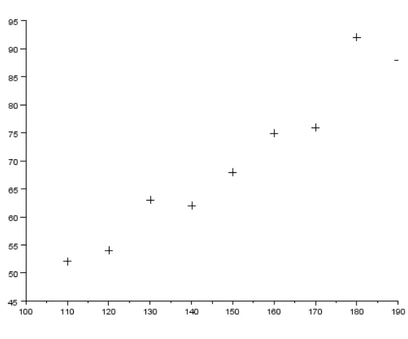
Scilab code Exa 9.1a Scatter Diagram

1 X = [100 110 120 130 140 150 160 170 180 190];

2 Y = [45 52 54 63 62 68 75 76 92 88];

3 plot2d(X , Y , -1) ;

4 disp(”A l i n e a r r e g r e s s i o n model s e e m s a p p r o p r i a t e ”)

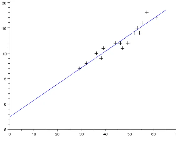
Scilab code Exa 9.2a Relative humidity and moisture content

1 A = [46 53 29 61 36 39 47 49 52 38 55 32 57 54 44];

2 B = [12 15 7 17 10 11 11 12 14 9 16 8 18 14 12];

3 plot2d(A , B , -1) ;

4 [X , Y ] = reglin(A , B ) ;

5 // d i s p (X) ;

6 // d i s p (Y) ;

(77)

(78)

(79)

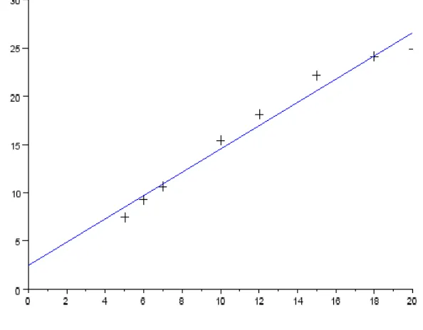
Figure 9.3: Moisture against Density

9 plot2d(p , q , 2) ;

Scilab code Exa 9.3a Moisture against Density

1 x = [5 6 7 10 12 15 18 20];

2 y = [7.4 9.3 10.6 15.4 18.1 22.2 24.1 24.8];

3 plot2d(x ,y , -1) ;

4

5 xbar = mean( x ) ;

6 ybar = mean( y ) ;

(80)

8 SxY = 0;

Scilab code Exa 9.4a Effect of speed on mileage

(81)

10

Scilab code Exa 9.4b Confidence interval estimate

1 x = [45 50 55 60 65 70 75];

2 y = [24.2 25.0 23.3 22.0 21.5 20.6 19.8];

(82)

6 SxY = 0;

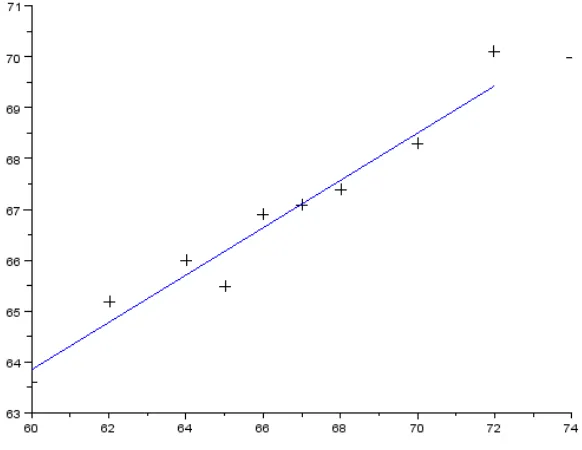
Scilab code Exa 9.4c Regression to the mean

1 x = [60 62 64 65 66 67 68 70 72 74];

(83)

(84)

(85)

Scilab code Exa 9.4d Motor vehicle deaths

(86)

(87)

(88)

Scilab code Exa 9.5a Height of son and father

1 x = [60 62 64 65 66 67 68 70 72 74];

2 y = [63.6 65.2 66 65.5 66.9 67.1 67.4 68.3 70.1 70];

3

6 n = 10;

7 SxY = 0;

8 for i = 1: n

9 SxY = SxY + ( x ( i ) * y ( i ) ) - ( xbar * ybar ) ;

10 end 11

12 Sxx = 0;

13 for i =1: n

14 Sxx = Sxx + ( x ( i ) * x ( i ) ) - ( xbar * xbar ) ;

15 end

16 SYY = 0;

17 for i =1: n

18 SYY = SYY + ( y ( i ) * y ( i ) ) - ( ybar * ybar ) ;

19 end

20 B = SxY / Sxx ;

21 A = ybar - ( B * xbar ) ;

22

23 SSR = (( Sxx * SYY ) - ( SxY * SxY ) ) / Sxx ;

24 R2 = 1 - ( SSR / SYY ) ;

(89)

Figure 9.5: Percentage of chemical used

(90)

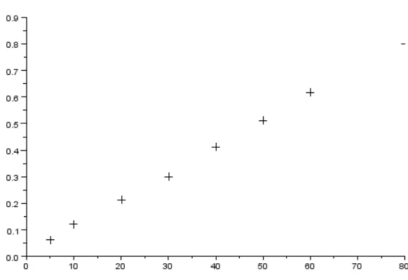
Scilab code Exa 9.7a Percentage of chemical used

1 x = [5 10 20 30 40 50 60 80];

(91)

Scilab code Exa 9.8b Distance vs Travel Time

1 x = [0.5 1 1.5 2 3 4 5 6 8 10];

2 y = [15 15.1 16.5 19.9 27.7 29.7 26.7 35.9 42 49.4];

3 for i =1:10

4 w ( i ) = 1/ x ( i ) ;

5 end

6 // d i s p (w)

7 n = 10;

8 p = zeros(2 ,2) ;

9 q = zeros(2 , 1) ;

10 p (1 , 1) = sum( w ) ;

11 p (1 ,2) = n ;

12 p (2 ,1) = n ;

13 p (2 ,2) = sum( x ) ;

14 for i =1:10

15 new ( i ) = w ( i ) * y ( i )

16 end 17

18 q (1 ,1) = -1*sum( new ) ;

19 q (2 ,1) = -1*sum( y ) ;

20 // d i s p ( p ) ;

21 // d i s p ( q ) ;

22 sol = linsolve(p , q ) ;

23 A = sol (1 ,1 ) ;

24 B = sol (2 ,1) ;

25 disp(A , ”A i s ”) ;

26 disp(B , ”B i s ”) ;

(92)

(93)

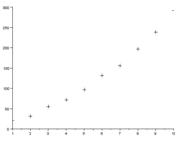
1 x = 1:1:10;

Scilab code Exa 9.10a Multiple Linear Regression

1 x1 = [679 1420 1349 296 6975 323 4200 633];

(94)

(95)

(96)

33 SSR = y ’;

Scilab code Exa 9.10c Diameter of a tree

(97)

17 // d i s p ( p r o 2 ) ; textbook gives the value as 19.26 , thus the

44

45 d i f f e r e n c e in the final answer .

Scilab code Exa 9.10d Estimating hardness

(98)

(99)

38 smallx = [1 , 0.15 , 1.15];

39 product = smallx * B ;

40 // d i s p ( p r o d u c t ) ;

41 n = 10;

42 k =2;

43 val = sqrt( SSR /( n -k -1) ) ;

44 // d i s p ( v a l ) ;

45

46 pro5 = smallx * pro3 ;

47 pro6 = pro5 * smallx ’;

48 pro7 = val *sqrt( pro6 ) * tvalue ;

49 // d i s p ( p r o 7 )

50 up = product + pro7 ;

51 low = product - pro7 ;

52 disp(” 95% c o n f i d e n c e i n t e r v a l i s from ”) ;

53 disp( up , ” t o ”, low ) ;

Scilab code Exa 9.11a Animal fsickalling

1 cancer = 84;

2 total = 111;

3 level = 250;

4 alpha = -1*log(( total - cancer ) / total ) / level ;

(100)

Chapter 10 Analysis of Variance

Scilab code Exa 10.3a Dependence of mileage on gas used

1 Xij = [220 251 226 246 260; 244 235 232 242 225; 252 272 250 238 256];

2 Xi = zeros(3 ,1) ;

3 n = 5;

4 m =3;

5 for i =1:3

6 for j =1:5

7 Xi ( i ) = Xi ( i ) + Xij (i , j ) ;

8 end

9 end

10 Xi = Xi / n ;

11 SSW = 0;

12 for i =1:3

13 for j = 1:5

14 SSW = SSW + (( Xij (i , j ) - Xi ( i ) ) ^2)

15 end

16 end

17 sigma1 = SSW /(( n * m ) -m ) ;

18 Xdotdot = sum( Xi ) / m ;

(101)

21 sigma2 = SSb /( m -1) ;

Scilab code Exa 10.3b Dependence of mileage on gas used

(102)

19 SSW = sum( X i j s q u a r e d ) - ( m * n *( Xdotdot ^2) ) - SSb ;

20 sigma1 = SSW /(( n * m ) -m ) ;

21 sigma2 = SSb /( m -1) ;

22 TS = sigma2 / sigma1 ;

23 disp( TS , ” V a l u e o f t h e t e s t s t a t i s t i c i s ”) ;

Scilab code Exa 10.3c Difference in GPA

(103)

27 disp( pvalue , ” The p−v a l u e i s ”)

19 alphahat = Xidot - meanhat ;

20 betahat = Xjdot - meanhat ;

(104)

(105)

26 SSe = SSe + ( X (i , j ) - Xidot ( i ) - Xjdot ( j ) + Xdotdot ) ^2;

27 end

28 end

29 N =( m -1) *( n -1) ;

30 TS1 = SSr * N /(( m -1) * SSe ) ;

31 TS2 = SSc * N /(( n -1) * SSe ) ;

32 pvaluec = 1 - cdff(”PQ”, TS1 , m -1 , N ) ;

33 pvaluer = 1 - cdff(”PQ”, TS2 , n -1 , N ) ;

34 // d i s p ( p v a l u e r , p v a l u e c ) ;

35 // d i s p ( TS1 , TS2 ) ;

36 disp( TS1 , ” The v a l u e o f t h e F−s t a t i s t i c f o r t e s t i n g t h a t t h e r e i s no row e f f e c t i s ”) ;

37 disp( pvaluec , ” The p−v a l u e f o r t e s t i n g t h a t t h e r e i s no row e f f e c t i s ”) ;

38

39 disp( TS2 , ” The v a l u e o f t h e F−s t a t i s t i c f o r t e s t i n g t h a t t h e r e i s no column e f f e c t i s ”) ;

(106)

Chapter 11 Goodness of Fit Tests and

Categorical Data Analysis

Scilab code Exa 11.2a Relation between death date and birth date

1 X = [90 100 87 96 101 86 119 118 121 114 113 106];

2 pi = ones(12 ,1) ;

3 pi = pi /12;

4 new = X .^2;

5 npi = sum( X ) * pi ;

6 T = sum( new ) ;

7 T = T / npi ;

8 T = T - sum( X ) ;

9 disp(”When t h e r e a r e 12 r e g i o n s ”)

10 disp( T (1) , ” The t e s t s t a t i s t i c i s ”)

11 pvalue = 1 - cdfchi(”PQ”,T (1) , 11) ;

13

14 X = [277 283 358 333];

15 pi = ones(4 ,1) ;

16 pi = pi /4;

17 new = X .^2;

(107)

20 T = T / npi ;

Scilab code Exa 11.2b Quality of bulbs

(108)

(109)

(110)

(111)

33 disp(” The n u l l h y p o t h e s i s i s r e j e c t e d a t t h e 5%

Scilab code Exa 11.4b Machine Breakdown and shift

(112)

27 end

Scilab code Exa 11.5a Lung cancer and smoking

(113)

21 NM = NM / n ;

Scilab code Exa 11.5b Females reporting abuse

(114)

15 NM = ones(2 ,4) ;

Scilab code Exa 11.6a Testing distribution of a population

1 X = [66 72 81 94 112 116 124 140 145 155];

2 D = 0 . 4 8 3 1 4 8 7 ;

3 n = 10;

4 Dgiven = 1.480;

(115)

7 if( Dstar > Dgiven )

8 disp(” N u l l h y p o t h e s i s i s r e j e c t e d a t 2 . 5% l e v e l o f s i g n i f i c a n c e ”)

9 else

10 disp(” N u l l h y p o t h e s i s i s a c c e p t e d a t 2 . 5% l e v e l o f s i g n i f i c a n c e ”)

(116)

Chapter 12 Non parametric Hypothesis

Tests

Scilab code Exa 12.2a testing the median

1 n = 200;

2 v = 120;

3 p =0.5;

4 if( v < ( n /2) )

5 pvalue = 2*cdfbin(”PQ”, v , n , p ,1 - p ) ;

6 else

7 pvalue = 2*cdfbin(”PQ”, n -v , n , p ,1 - p ) ;

8 9 end

10 disp( pvalue , ” P v a l u e i s ”) ;

Scilab code Exa 12.2b testing the median

1 n = 80;

2 v = 28;

(117)

4

Scilab code Exa 12.3b Signed Rank Test

(118)

Scilab code Exa 12.3c Determining Population Distribution

Scilab code Exa 12.4a Treatments against corrosion

(119)

(120)

25 result = 2*min( prob (n ,m , t ) , 1 - prob (n ,m ,t -1) ) ;

Scilab code Exa 12.4c Finding p value

1 ans = pval (5 ,6 ,21) ;

2 disp(ans)

Scilab code Exa 12.4d Comparing production methods

1 ans = pval (9 ,13 ,72) ;

2 disp(ans)

Scilab code Exa 12.4e Determining p value

1 n1 =5;

2 m1 = 6;

3

4 t1 =21;

5 num1 = n1 *( n1 + m1 +1) /2;

6 d1 =abs( t1 - num1 ) ;

7 val = d1 /sqrt( n1 * m1 *( n1 + m1 +1) /12) ;

8 // d i s p ( d1 , ” d i s ” )

9 // d i s p ( v a l , ” v a l i s ” )

10 pval = 2*(1 -cdfnor(”PQ”, val , 0 ,1) ) ;

11 disp( pval , ” The p−v a l u e f o r e g 1 2 . 4 a i s ”)

12 n2 =9;

13 m2 = 13;

(121)

(122)

23 ans1 = ans1 + proba ( n1 , m1 , i ) ;

24 // d i s p ( p r o b a ( n , m, i ) ) ;

25 // d i s p ( a n s 1 )

26 end

27 if( ans1 <0.5)

28 pvalue1 = 2* ans1 ;

29 else

30 pvalue1 = 2*(1 - ans1 ) ;

31 end

32 disp( pvalue1 , ”P−v a l u e i s ”)

Scilab code Exa 12.5c Determining p value

1 u = 61;

2 sigma = 5.454;

3 r =75;

4 val = cdfnor(”PQ”, (r - u ) / sigma , 0 ,1) ;

5 if( val >0.5)

6 pvalue = 2*(1 - val ) ;

7 else

8 pvalue = 2* val ;

9 end

(123)

Chapter 13 Quality Control

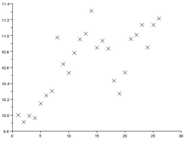
Scilab code Exa 13.2a Steel shaft diameter

1 X = [3.01 2.97 3.12 2.99 3.03 3.02 3.10 3.14 3.09 3.20];

2 Y = 1:1:10;

3 u = 3;

4 sigma = 0.1;

5 n =4;

6 ucl = u + (3* sigma /sqrt( n ) ) ;

7 lcl = u - (3* sigma /sqrt( n ) ) ;

8 Z = 0 . 1 : 0 . 1 : 1 0 ;

9 P = ones(1 ,100) ;

10 Q = ones(1 ,100) ;

11 P = P * ucl ;

12 Q = Q * lcl ;

13 plot2d(Y , X , -2) ;

14 plot2d(Z , P , 1) ;

15 plot2d(Z , Q , 1) ;

16 // d i s p ( s i z e ( Z ) ) ;

17 // d i s p ( s i z e (P) ) ;

18 disp( ucl , ’ u c l i s ’) ;

(124)

Scilab code Exa 13.2b unknown mean and variance

1 Xbar = [3.01 2.97 3.12 2.99 3.03 3.02 3.10 3.14 3.09 3.20];

2 S = [0.12 0.14 0.08 0.11 0.09 0.08 0.15 0.16 0.13 0.16];

3 c = [ 0 . 7 9 7 8 8 4 9 0. 88 6 22 66 0 .9 2 13 18 1 0. 9 39 98 5 1 0 .9 51 5 33 2 0. 95 9 36 8 4 0 . 96 50 3 09 0 .9 69 3 10 3 0 . 9 7 2 6 5 9 6 ] ;

4 n =4;

5 Xbarbar = mean( Xbar ) ;

6 Sbar =mean( S ) ;

7 lcl = Xbarbar - (3* Sbar /(sqrt( n ) * c (n -1) ) ) ;

8 ucl = Xbarbar + (3* Sbar /(sqrt( n ) * c (n -1) ) ) ;

9 // d i s p ( l c l , ”LCL i s ” )

10 // d i s p ( u c l , ”UCL i s ” )

11 u = Xbarbar ;

12 sigma = Sbar / c (n -1) ;

13 // d i s p ( u ) ;

14 // d i s p ( s i g m a ) ;

15 // d i s p ( Sbar , c ( 4 ) ) ;

16 prob = cdfnor(”PQ”, 3.1 , u , sigma ) - cdfnor(”PQ”, 2.9 , u , sigma ) ;

17 disp( prob *100 , ” P e r c e n t a g e o f t h e i t e m s t h a t w i l l meet t h e s p e c i f i c a t i o n s i s ”)

(125)

(126)

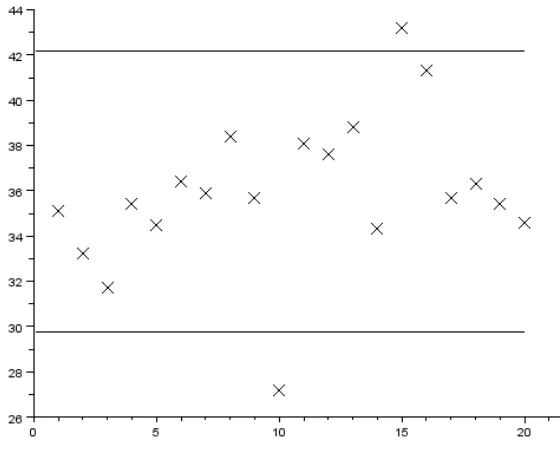
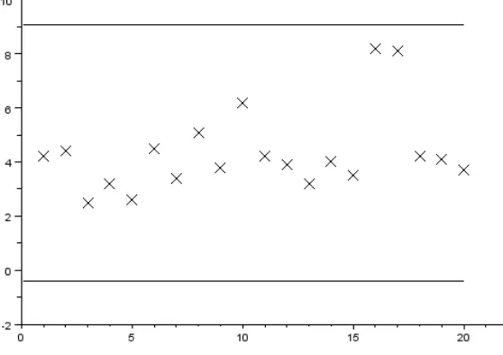
Figure 13.2: determining control limits

1 Xbar = [35.1 33.2 31.7 35.4 34.5 36.4 35.9 38.4 35.7 27.2 38.1 37.6 38.8 34.3 43.2 41.3 35.7 36.3

35.4 34.6];

2 S = [4.2 4.4 2.5 3.2 2.6 4.5 3.4 5.1 3.8 6.2 4.2 3.9 3.2 4 3.5 8.2 8.1 4.2 4.1 3.7];

3 c = [ 0 . 7 9 7 8 8 4 9 0. 88 6 22 66 0 .9 2 13 1 81 0. 9 39 9 85 1 0 .9 51 5 33 2 0. 95 9 36 8 4 0 . 96 50 3 09 0 .9 69 3 10 3 0 . 9 7 2 6 5 9 6 ] ;

4 Y = 1:1:20;

5 n =5;

6 Z = 0 . 1 : 0 . 1 : 2 0 ;

7 Xbarbar = mean( Xbar ) ;

8 Sbar = mean( S ) ;

9 lclX = Xbarbar - (3* Sbar /(sqrt( n ) * c (n -1) ) ) ;

10 uclX = Xbarbar + (3* Sbar /(sqrt( n ) * c (n -1) ) ) ;

11 val1 = 1/ c (n -1) ;

(127)

(128)

6 val = sqrt( Fbar *(1 - Fbar ) / n ) ;

Scilab code Exa 13.5a Control during production of cars

(129)

11 total = total - X ( i ) ;

given in the book is 82.56. The values of UCL and LCL

36 change a c c o r d i n g l y .

Scilab code Exa 13.6b Service Time

(130)

84];

Scilab code Exa 13.6c Exponentially weighted moving average control

(131)

(132)

11 W = zeros(26) ;

Scilab code Exa 13.6d Finding control limit

(133)

10 S ( i ) = max( S (i -1) + Y (i -1) , 0) ;

11 end

12 disp(S , ” S i s ”)

13 cl = B * sig ;

14 disp( cl )

15 answer =100;

16 for i =1:9

17 if( S ( i ) > cl )

18 answer = i ;

19 end

20 end

21 disp(” The mean h a s i n c r e a s e d a f t e r o b s e r v i n g t h e ”)

22 disp( answer -1) ;

(134)

Chapter 14 Life Testing

Scilab code Exa 14.3a Lifetime of a transistor

1 total =50;

2 failure = 15;

3 alpha = 0.05;

4 t =525;

5 val1 = cdfchi(”X”, 2* failure , alpha /2 , 1 -( alpha /2) ) ;

6 val2 = cdfchi(”X”, 2* failure , 1 - alpha /2 , ( alpha /2) ) ;

7

8 int1 = 2* t / val1 ;

9 int2 = 2* t / val2 ;

10 disp(” The 95% c o n f i d e n c e i n t e r v a l i s ”) ;

11 disp( int2 ) ;

12 disp( int1 , ” t o ”) ;

13

14 // The c o n f i d e n c e i n t e r v a l i s from 2 2 . 3 5 t o 6 2 . 1 7 w h e r e a s my s o l u t i o n i n S c i l a b i s 2 2 . 3 5 t o 6 2 . 5 3

15 because of the d i f f e r e n c e in the value of chi -square

(0.975 , 30) . The textbook says the value is 16.89

(135)

Scilab code Exa 14.3b Lifetime of Battery

1 t = 1800;

2 theta = 150;

3 r =20;

4 pvalue = cdfchi(”PQ”,2* t / theta , 2* r ) ;

5 disp( pvalue , ”P−v a l u e i s ”)

Scilab code Exa 14.3c One at a time sequential test

1 T = 500;

2 alpha = 0.05;

3 r = 10;

4 val1 = cdfchi(”X”, 2* r , 1 - alpha /2 , alpha /2) ;

5 val2 = cdfchi(”X”, 2* r , alpha /2 , 1 - alpha /2) ;

6 int1 = 2* T / val1 ;

7 int2 = 2* T / val2 ;

8 disp(” The 95% c o n f i d e n c e i n t e r v a l i s ”) ;

9 disp( int1 ) ;

10 disp( int2 , ” t o ”) ;

11

12 // The c o n f i d e n c e i n t e r v a l i s from 2 9 . 2 7 t o 1 0 3 . 5 2 w h e r e a s my s o l u t i o n i n S c i l a b i s 2 9 . 2 6 5 7 7 4 t o

13 1 04 .2 6 68 3 because of the d i f f e r e n c e in the value of chi -square(0.975 , 30) . The textbook says the value is

(136)

Scilab code Exa 14.3d Lifetime of semiconductors

1 r = 30;

2 T = 600;

3 theta = 25;

4 val1 = cdfchi(”PQ”, 2* T / theta , 2* r ) ;

5 val2 = 1 - cdfchi(”PQ”, 2* T / theta , 2*( r +1) ) ;

6 pvalue = min( val1 , val2 ) ;

7 disp( pvalue , ” The p v a l u e i s ”) ;

8 disp(”H0 would be a c c e p t e d when t h e s i g n i f i c a n c e l e v e l i s 0 . 1 0 ”) ;

Scilab code Exa 14.3e Bayes estimator

1 X = [5 7 6.2 8.1 7.9 15 18 3.9 4.6 5.8];

2 Y = [3 3.2 4.1 1.8 1.6 2.7 1.2 5.4 10.3 1.5];

3 t = sum( X ) +sum( Y ) ;

4 R =10;

5 a = 20;

6 b = 2;

7 estimate = ( R + b ) /( a + t ) ;

8 disp( estimate , ” Bayes e s t i m a t e o f lambda i s ”) ;

Scilab code Exa 14.4a Lifetime of items produced by two plants

1 Xlife = 420;

2 Ylife = 510;

3 Xnum = 10;

4 Ynum =15;

5 ts = Xlife * Ynum /( Ylife * Xnum ) ;

6 disp( ts , ” The v a l u e o f t h e t e s t s t a t i s t i c i s ”) ;

(137)

9 disp( pvalue , ” The p−v a l u e i s ”) ;

Probability And Statistics For Engineers (3)

Scilab Textbook Companion for

Probability And Statistics For Engineers And

Scientists

by S. M. Ross

1

Created by

Deeksha Sinha

Dual Degree

Electrical Engineering

IIT Bombay

College Teacher

None

Cross-Checked by

Mukul R. Kulkarni

August 10, 2013

Book Description

Contents

List of Figures

Chapter 2

Descriptive Statistics

Chapter 3

Elements Of Probability

Chapter 4

Random Variables And

Expectation

Chapter 5

Special Random Variables

Chapter 6

Distribution of Sampling

Statistics

Chapter 7

Parameter Estimation

Chapter 8

Hypothesis Testing

Chapter 9

Regression

Chapter 10

Analysis of Variance

Chapter 11

Goodness of Fit Tests and

Categorical Data Analysis

Chapter 12

Non parametric Hypothesis

Tests

Chapter 13

Quality Control

Chapter 14

Life Testing