LAMPIRAN A : MENTERJEMAHKAN SETIAP LANGKAH DEMI LANGKAH KE BAHASA MATHEMATICA 9

LAMPIRAN A : MENTERJEMAHKAN SETIAP LANGKAH DEMI

LANGKAH KE BAHASA MATHEMATICA 9

Persaman gerak untuk

θ

1

adalah

(𝑚

1

+ 𝑚

2

+ 𝑚

3

)𝑙

1

𝜃̈

1

+ (𝑚

2

+ 𝑚

3

)𝑙

2

𝑐𝑜𝑠(𝜃

1

− 𝜃

2

)𝜃̈

2

+ 𝑚

3

𝑙

3

𝑐𝑜𝑠(𝜃

1

−

𝜃

3

)𝜃̈

3

+ (𝑚

2

+ 𝑚

3

)𝑙

2

𝜃̇

22

𝑠𝑖𝑛(𝜃

1

− 𝜃

2

) + 𝑚

3

𝑙

3

𝜃̇

32

𝑠𝑖𝑛(𝜃

1

− 𝜃

3

) + (𝑚

1

+ 𝑚

2

+

𝑚

3

)𝑔 𝑠𝑖𝑛𝜃

1

= 0

(2.19)

Diubah dalam program menjadi

g (m1+m2+m3) Sin[θ1[t]]+θ2’[t]^2 l2 (m2+m3) Sin[θ1[t]

-θ2[t]]+θ3’[t]^2 l3 m3 Sin[θ1[t]-θ3[t]]+l1 m1 θ1’’[t]+(m2+m3)

Penyelesaian persamaan differensial

triple

pendulum:

sol=NDSolve[eqns, (θ1,θ2}, {t,0,p}, Maxsteps->Infinity, PrecisionGoal->4];pq=sol[[1,1,2,1,1,2]];

Posisi Persamaan pendulum :

pos2[t_]:={(l1 Sin[θ1[t]]+l2 Sin[θ2[t]]),(-l1 Cos[θ1[t]]-l2

Cos[θ2[t]])};

pos3[t_]:={(l1 Sin[θ1[t]]+l2 Sin[θ2[t]]+l3 Sin[θ3[t]]),(-l1

Cos[θ1[t]]-l2 Cos[θ2[t]]-l3 Cos[θ3[t]])};

Jejak persamaan Gerak Pendulum dalam simulasi:

path=ParametricPlot[Evaluate[pos3[t]/.sol[[1]],{t,p-Batasan dalam visualiasi Pendulum :

Tombol Pemilihan Grafik hasil animasi Pendulum :

Switch[plottype,

(*Tampilan plot simpangan x m1 dan m2 terhadap t*)

x1x2, Plot[{g1[t], g2[t]}, {t,0,p},

MaxRecursion->ControlActive[3, 4], PlotStyle->{Green, Blue}, Axes->False,PlotLabel->Style{“x(t)vs t”, “Label”], PlotRange

->{{pq-25,pq}, Automatic}, ImageSize->{420, 150},

AspectRatio->32/100.],

(*Tampilan plot simpangan y m1 dan m2 terhadap t*)

y1y2, Plot[{g1[t], g2[t]}, {t,0,p},

MaxRecursion->ControlActive[3, 4], PlotStyle->{Green, Blue}, Axes->False,PlotLabel->Style{“x(t)vs t”, “Label”], PlotRange

->{{pq-25,pq}, Automatic}, ImageSize->{420, 150},

AspectRatio->32/100.],

(*Tampilan plot simpangan x m2 dan m3 terhadap t*)

x2x3, Plot[{g1[t], g2[t]}, {t,0,p},

MaxRecursion->ControlActive[3, 4], PlotStyle->{Blue, Red},

Axes->False,PlotLabel->Style{“x(t)vs t”, “Label”], PlotRange

->{{pq-25,pq}, Automatic}, ImageSize->{420, 150},

AspectRatio->32/100.],

(*Tampilan plot simpangan y m2 dan m3 terhadap t*)

y2y3, Plot[{g1[t], g2[t]}, {t,0,p},

MaxRecursion->ControlActive[3, 4], PlotStyle->{Blue, Red},

Axes->False,PlotLabel->Style{“x(t)vs t”, “Label”], PlotRange

->{{pq-25,pq}, Automatic}, ImageSize->{420, 150},

AspectRatio->32/100.],

(*Tampilan plot simpangan θ m1 dan m2 terhadap t*)

θ1θ2, Plot[{g1[t], g2[t]}, {t,0,p},

->{{pq-25,pq}, Automatic}, ImageSize->{420, 150}, AspectRatio->32/100.],

(*Tampilan plot simpangan θ m2 dan m3 terhadap t*)

θ2θ3, Plot[{g1[t], g2[t]}, {t,0,p},

MaxRecursion->ControlActive[3, 4], PlotStyle->{Blue, Red},

Axes->False,PlotLabel->Style{“θ(t)vs t”, “Label”], PlotRange

->{{pq-25,pq}, Automatic}, ImageSize->{420, 150},

AspectRatio->32/100.],

(*Tampilan Plot x1 vs y1*)

x1y1,

ParametricPlot[{g1[t],g2[t]},{t,0,p},MaxRecursion-

>ControlActive[3,4],Axes->False,PlotLabel->Rown[{Subscript[x,1],” vs “,

Subscript[y,1]}],PlotRange->{{-3Pi/4,3Pi/4}, Automatic},

ImageSize->{420,150},PlotStyle->Darker[Green,.1],AspectRatio->32/100.],

(*Tampilan Plot x2 vs y2*)

x2y2,

ParametricPlot[{g1[t],g2[t]},{t,0,p},MaxRecursion-

>ControlActive[3,4],Axes->False,PlotLabel->Rown[{Subscript[x,2],” vs “, Subscript[y,2]}],PlotRange

->{{-3Pi/2,3Pi/2}, Automatic},

ImageSize->{420,150},PlotStyle->Darker[Blue,.1],AspectRatio->32/100.],

(*Tampilan Plot x3 vs y3*)

x3y3,

ParametricPlot[{g1[t],g2[t]},{t,0,p},MaxRecursion-

>ControlActive[3,4],Axes->False,PlotLabel->Rown[{Subscript[x,3],” vs “, Subscript[y,3]}],PlotRange

->{{-3Pi/2,3Pi/2}, Automatic},

ImageSize->{420,150},PlotStyle->Darker[Blue,.1],AspectRatio->32/100.],

(*Tampilan Plot θ1 vs θ2*)

θθ, ParametricPlot[{g1[t],g2[t]},{t,0,p},MaxRecursion -

->{{-Pi,Pi}, Automatic}, ImageSize->{420,150},ColorFunction->(Blend[{Blue, Green}, #1]&),AspectRatio->32/100.],

(*Tampilan Plot θ2 vs θ3*)

θϕ, ParametricPlot[{g1[t],g2[t]},{t,0,p},MaxRecursion -

>ControlActive[3,4],Axes->False,PlotLabel->Rown[{Subscript[θ,2],” vs “, Subscript[θ,3]}],PlotRange

->{{-Pi,Pi}, Automatic},

ImageSize->{420,150},ColorFunction->(Blend[{Red, Blue}, #1]&),AspectRatio->32/100.],

(*Tampilan plot ω1 vs θ1*)

θθPrime1, ParametricPlot[{g1[t], g2[t]}, {t,0,p}, MaxRecursion

->ControlActive[3,4],

Axes->False,PlotLabel->Row[{Subscript[OverDot[θ],1],” vs “,Subscript[θ,1]}],Plot Range->{{-Pi,Pi}, Automatic},ImageSize{420,150},AspectRatio->32/100., PlotStyle->Darker[Green,.2]],

(*Tampilan plot ω2 vs θ2*)

θθPrime2, ParametricPlot[{g1[t], g2[t]}, {t,0,p}, MaxRecursion

->ControlActive[3,4],

Axes->False,PlotLabel->Row[{Subscript[OverDot[θ],2],” vs “,Subscript[θ,2]}],PlotRange ->{{-Pi,Pi}, Automatic},ImageSize{420,150},AspectRatio->32/100., PlotStyle->Darker[Blue,.2]],

(*Tampilan plot ω3 vs θ3*)

θθPrime2, ParametricPlot[{g1[t], g2[t]}, {t,0,p}, MaxRecursion

->ControlActive[3,4],

Style[“***********************************************”, Bold,16, Darker[Black, .1], “Label”],

Style[“PENDULUM NONLINIER”, Bold, 18, Darker[Black, .1], “Label”],

Style[“******************************************”, Bold, 12, Darker[Black, .1], “Label”],

Style[“ “, Bold, 12, Darker[Green,.8], “Label”],

Style[“Parameter Pendulum”,”Subsection”, Bold, 12,

Darker[Black,.1], “Label”],

Tampilan Parameter massa pendulum hijau, biru, merah, panjang pendulum hijau,

biru, merah, gravitasi, sudut pendulum hijau, biru, merah, kecepatan sudut pendulum

hijau, biru, merah, dan waktu (Berurutan):

{{m1, 1, “Green mass (m1)”},1,5,ImageSize->Tiny,

ContinuousAction->False, Appearance->”Labeled”},

{{m2,1,”Blue mass (m2)”},1,5, ImageSize->Tiny,

ContinuousAction->False, Appearance->”Labeled”},

{{m3,1,”Red mass (m3)”},1,5, ImageSize->Tiny,

ContinuousAction->False, Appearance->”Labeled”},

{{l1,1,”Green length (l1)”},1,5,ImageSize->Tiny,

ContinuousAction->False, Appearance->”Labeled”},

{{l2,1,”Blue length (l2)”},1,5, ImageSize->Tiny,

ContinuousAction->False, Appearance->”Labeled”},

{{l3,1,”Red length (l3)”},1,5, ImageSize->Tiny,

ContinuousAction->False, Appearance->”Labeled”},

{{g,1,”Gravity (g)”},1,9.8, ImageSize->Tiny, ContinuousAction->False, Appearance->”Labeled”},

Delimiter,

Style[“Kondisi Awal”, “Subsection”, Bold, 12,

Darker[Black,.1],”Label”],

{{init1,Pi/2,”green angle(θ1)

“},-Pi/2, Pi/2, Appearance->”Labeled”, ImageSize->Tiny},

{{init2,0,”blue angle(θ2)

{{init3,0,”red angle(θ3)

“},-Pi/2, Pi/2, Appearance->”Labeled”, ImageSize->Tiny},

{{initprime1,0,”green velocity(ω1)”},0,5,ImageSize

->Tiny,Appearance->”Labeled”},

{{initprime2,0,”blue velocity(ω2)”},0,

5,ImageSize->Tiny,Appearance->”Labeled”},

{{initprime3,0,”red velocity(ω3)”},0,5,ImageSize

->Tiny,Appearance->”Labeled”},

m3”, y2y3->” Simpangan y m2 dan m3”,θ1θ2->”Sensitivitas Kondisi

Awal θ1 dan θ2”, θ2θ3->”Sensitivitas Kondisi Awal θ2 dan

θ3”,x1y1->”x1 vs. y1”, x2y2->”x2 vs. y2”, x3y3->”x3 vs. y3”,θθ->”θ1

vs. θ2”, θϕ->”θ2 vs. θ3”, θθprime1->” 𝜃̇₁ vs θ1”, θθprime2->” 𝜃̇₂ vs

θ2”, θθprime3->” 𝜃̇3 vs θ3”} ”},ControlType->PopupMenu}

Tombol untuk menganimasikan pendulum terhadap waktu:

{{p,0.001,”Animasi”},0.001,100,1.0, ControlType->Trigger},

AutorunSequencing->All,TrackedSymbols:->Manipulate,Initialization:->Get[“Barcharts”],

LAMPIRAN B: LISTING PROGRAM SIMULASI GERAK TRIPLE

PENDULUM NONLINIER

Berikut ini merupakan listing program untukanimasi dan visualisasi gerakan triple pendulum nonlinier

(*Penentuan Variabel-variabel dan konstanta-konstanta*)

sol=NDSolve[eqns, (θ1,θ2}, {t,0,p}, Maxsteps->Infinity, PrecisionGoal->4];pq=sol[[1,1,2,1,1,2]];

pos1[t_]:={l1 Sin[θ1[t]],-l1 Cos[θ1[t]]};

pos2[t_]:={(l1 Sin[θ1[t]]+l2 Sin[θ2[t]]),(-l1 Cos[θ1[t]]-l2

Cos[θ2[t]])};

pos3[t_]:={(l1 Sin[θ1[t]]+l2 Sin[θ2[t]]+l3 Sin[θ3[t]]),(-l1

Cos[θ1[t]]-l2 Cos[θ2[t]]-l3 Cos[θ3[t]])};

path=ParametricPlot[Evaluate[pos3[t]/.sol[[1]],{t,p-

path1=ParametricPlot[Evaluate[pos2[t]/.sol[[1]],{t,p-p/5,p},

Darker[Green,.2],Line[{{0, 0}, First@Evaluate[pos1[pq]/.sol]}], Disk[First@Evaluate[pos1[pq]/.sol,.2],ImageSize->{320, Sin[θ2[t]],y1y2,(-l1 Cos[θ1[t]]-l2 Cos[θ2[t]]),x2x3,(l1

Sin[θ1[t]+l2 Sin[θ2[t]]+l3 Sin[θ3[t]]),y2y3,(-l1 Cos[θ1[t]-l2 Cos[t]]-l3

Cos[t]]),x1y1,pos1[t][[2]],x2y2,pos2[t][[2]],pos3[t][[2]],θ1θ2, θ2[t],θ2θ3,θ3[t],θθ,θ2[t],θϕ,θ3[t],θθprime1,θ1’[t],θθprime2, θ2’[t],θθprime3,θ3’[t],_,1]/.sol[[1]];

Switch[plottype,

(*Tampilan plot simpangan x m1 dan m2 terhadap t*)

x1x2, Plot[{g1[t], g2[t]}, {t,0,p},

MaxRecursion->ControlActive[3, 4], PlotStyle->{Green, Blue}, Axes->False,PlotLabel->Style{“x(t)vs t”, “Label”],

PlotRange->{{pq-25,pq}, Automatic}, ImageSize->{420, 150},

(*Tampilan plot simpangan y m1 dan m2 terhadap t*)

y1y2, Plot[{g1[t], g2[t]}, {t,0,p},

MaxRecursion->ControlActive[3, 4], PlotStyle->{Green, Blue}, Axes->False,PlotLabel->Style{“x(t)vs t”, “Label”], PlotRange

->{{pq-25,pq}, Automatic}, ImageSize->{420, 150},

AspectRatio->32/100.],

(*Tampilan plot simpangan x m2 dan m3 terhadap t*)

x2x3, Plot[{g1[t], g2[t]}, {t,0,p},

MaxRecursion->ControlActive[3, 4], PlotStyle->{Blue, Red},

Axes->False,PlotLabel->Style{“x(t)vs t”, “Label”], PlotRange

->{{pq-25,pq}, Automatic}, ImageSize->{420, 150},

AspectRatio->32/100.],

(*Tampilan plot simpangan y m2 dan m3 terhadap t*)

y2y3, Plot[{g1[t], g2[t]}, {t,0,p},

MaxRecursion->ControlActive[3, 4], PlotStyle->{Blue, Red},

Axes->False,PlotLabel->Style{“x(t)vs t”, “Label”], PlotRange

->{{pq-25,pq}, Automatic}, ImageSize->{420, 150},

AspectRatio->32/100.],

(*Tampilan plot simpangan θ m1 dan m2 terhadap t*)

θ1θ2, Plot[{g1[t], g2[t]}, {t,0,p},

MaxRecursion->ControlActive[3, 4], PlotStyle->{Green, Blue}, Axes->False,PlotLabel->Style{“θ(t)vs t”, “Label”], PlotRange

->{{pq-25,pq}, Automatic}, ImageSize->{420, 150},

AspectRatio->32/100.],

(*Tampilan plot simpangan θ m2 dan m3 terhadap t*)

θ2θ3, Plot[{g1[t], g2[t]}, {t,0,p},

MaxRecursion->ControlActive[3, 4], PlotStyle->{Blue, Red},

Axes->False,PlotLabel->Style{“θ(t)vs t”, “Label”], PlotRange

->{{pq-25,pq}, Automatic}, ImageSize->{420, 150},

(*Tampilan Plot x1 vs y1*)

x1y1,

ParametricPlot[{g1[t],g2[t]},{t,0,p},MaxRecursion-

>ControlActive[3,4],Axes->False,PlotLabel->Rown[{Subscript[x,1],” vs “, Subscript[y,1]}],PlotRange

->{{-3Pi/4,3Pi/4}, Automatic},

ImageSize->{420,150},PlotStyle->Darker[Green,.1],AspectRatio->32/100.],

(*Tampilan Plot x2 vs y2*)

x2y2,

ParametricPlot[{g1[t],g2[t]},{t,0,p},MaxRecursion-

>ControlActive[3,4],Axes->False,PlotLabel->Rown[{Subscript[x,2],” vs “, Subscript[y,2]}],PlotRange

->{{-3Pi/2,3Pi/2}, Automatic},

ImageSize->{420,150},PlotStyle->Darker[Blue,.1],AspectRatio->32/100.],

(*Tampilan Plot x3 vs y3*)

x3y3,

ParametricPlot[{g1[t],g2[t]},{t,0,p},MaxRecursion-

>ControlActive[3,4],Axes->False,PlotLabel->Rown[{Subscript[x,3],” vs “, Subscript[y,3]}],PlotRange

->{{-3Pi/2,3Pi/2}, Automatic},

ImageSize->{420,150},PlotStyle->Darker[Blue,.1],AspectRatio->32/100.],

(*Tampilan Plot θ1 vs θ2*)

θθ, ParametricPlot[{g1[t],g2[t]},{t,0,p},MaxRecursion -

>ControlActive[3,4],Axes->False,PlotLabel->Rown[{Subscript[θ,1],” vs “, Subscript[θ,2]}],PlotRange

->{{-Pi,Pi}, Automatic},

ImageSize->{420,150},ColorFunction->(Blend[{Blue, Green}, #1]&),AspectRatio->32/100.],

(*Tampilan Plot θ2 vs θ3*)

θϕ, ParametricPlot[{g1[t],g2[t]},{t,0,p},MaxRecursion -

>ControlActive[3,4],Axes->False,PlotLabel->Rown[{Subscript[θ,2],” vs “, Subscript[θ,3]

}],PlotRange->{{-Pi,Pi}, Automatic},

(*Tampilan plot ω1 vs θ1*)

θθPrime1, ParametricPlot[{g1[t], g2[t]}, {t,0,p}, MaxRecursion

->ControlActive[3,4],

Axes->False,PlotLabel->Row[{Subscript[OverDot[θ],1],” vs “,Subscript[θ ,1]}],PlotRange->{{-Pi,Pi}, Automatic},ImageSize{420,150},AspectRatio->32/100., PlotStyle->Darker[Green,.2]],

(*Tampilan plot ω2 vs θ2*)

θθPrime2, ParametricPlot[{g1[t], g2[t]}, {t,0,p},

MaxRecursion->ControlActive[3,4],

Axes->False,PlotLabel->Row[{Subscript[OverDot[θ],2],” vs “,Subscript[θ,2]}],PlotRange ->{{-Pi,Pi}, Automatic},ImageSize{420,150},AspectRatio->32/100., PlotStyle->Darker[Blue,.2]],

(*Tampilan plot ω3 vs θ3*)

θθPrime2, ParametricPlot[{g1[t], g2[t]}, {t,0,p},

MaxRecursion->ControlActive[3,4],

Axes->False,PlotLabel-Style[“ANIMASI GERAK TRIPLE”, Bold, 18, Darker[Black,.1], “Label”],

Style[“***********************************************”,

Bold,16, Darker[Black, .1], “Label”],

Style[“PENDULUM NONLINIER”, Bold, 18, Darker[Black, .1], “Label”],

Style[“******************************************”, Bold, 12, Darker[Black, .1], “Label”],

Style[“ “, Bold, 12, Darker[Green,.8], “Label”],

Style[“Parameter Pendulum”,”Subsection”, Bold, 12,

{{m1, 1, “Green mass (m1)”},1,5,ImageSize->Tiny,

ContinuousAction->False, Appearance->”Labeled”},

{{m2,1,”Blue mass (m2)”},1,5, ImageSize->Tiny,

ContinuousAction->False, Appearance->”Labeled”},

{{m3,1,”Red mass (m3)”},1,5, ImageSize->Tiny,

ContinuousAction->False, Appearance->”Labeled”},

{{l1,1,”Green length (l1)”},1,5,ImageSize->Tiny,

ContinuousAction->False, Appearance->”Labeled”},

{{l2,1,”Blue length (l2)”},1,5, ImageSize->Tiny,

ContinuousAction->False, Appearance->”Labeled”},

{{l3,1,”Red length (l3)”},1,5, ImageSize->Tiny,

ContinuousAction->False, Appearance->”Labeled”},

{{g,1,”Gravity (g)”},1,9.8, ImageSize->Tiny, ContinuousAction->False, Appearance->”Labeled”},

Delimiter,

Style[“Kondisi Awal”, “Subsection”, Bold, 12,

Darker[Black,.1],”Label”],

{{init1,Pi/2,”green angle(θ1)

“},-Pi/2, Pi/2, Appearance->”Labeled”, ImageSize->Tiny},

{{init2,0,”blue angle(θ2)

“},-Pi/2, Pi/2, Appearance->”Labeled”, ImageSize->Tiny},

{{init3,0,”red angle(θ3)

“},-Pi/2, Pi/2, Appearance->”Labeled”, ImageSize->Tiny},

{{initprime1,0,”green velocity(ω1)”},0,5,ImageSize

->Tiny,Appearance->”Labeled”},

{{initprime2,0,”blue velocity(ω2)”},0,5,ImageSize

->Tiny,Appearance->”Labeled”},

{{initprime3,0,”red velocity(ω3)”},0,5,ImageSize

m3”, y2y3->” Simpangan y m2 dan m3”,θ1θ2->”Sensitivitas Kondisi

Awal θ1 dan θ2”, θ2θ3->”Sensitivitas Kondisi Awal θ2 dan

θ3”,x1y1->”x1 vs. y1”, x2y2->”x2 vs. y2”, x3y3->”x3 vs. y3”,θθ->”θ1

vs. θ2”, θϕ->”θ2 vs. θ3”, θθprime1->” 𝜃̇1 vs θ1”, θθprime2->” 𝜃̇2 vs

θ2”, θθprime3->” 𝜃̇₃ vs θ3”},

ControlType->PopupMenu},{{p,0.001,”Animasi”},0.001,100,1.0, ControlType->Trigger}, AutorunSequencing->All,TrackedSymbols:->Manipulate,Initialization:->Get[“Barcharts”],

LAMPIRAN C: PENJABARAN PERSAMAAN GERAK SISTEM TRIPLE

PENDULUM NONLINIER

Koordinat

–

koordinat posisi tiap pendulum :

x

1

= l

1

+ l

2

+ l

3

–

l

1

cos θ

1

(2.2)

Kemudian, setiap koordinat diatas akan diturunkan terhadap waktu untuk

memperoleh kecepatan. Hasil dari turunan menghasilkan

𝑥̇

1

= −𝑙

1

𝜃̇

1

sin 𝜃

1

trigonometri untuk selisih dua sudut diperoleh energi kinetik :



T =

1

Energi potensial diperoleh dengan mensubsitusikan persamaan 2.2, 2.4, 2.6 ke

persamaan 2.9 :

V =

m

1

gx

1

+ m

2

gx

2

+ m

3

gx

3

=

m

1

g (l

1

+ l

2

+ l

3

–

l

1

cos θ1

) + m

2

g (l

1

+ l

2

+ l

3

–

l

1 cos θ1

–

l

2cos θ2

) + m

3

g (l

1

+ l

2

Sehingga Fungsi Lagrangian

Triple

Pendulum Nonlinier:

Persamaan diatas adalah Fungsi Lagrangian dari

triple

pendulum, persamaan diatas

akan diselesaikan dengan persamaan Lagrange agar diperoleh posisi masing-masing

pendulum.

Persamaan Lagrange dirumuskan sebagai berikut:

𝑑

𝑚

1

𝑙

12

𝜃̈

1

+ 𝑚

2

𝑙

12

𝜃̈

1

+ 𝑚

3

𝑙

12

𝜃̈

1

+ 𝑚

2

𝑙

1

𝑙

2

𝜃̈

2

𝑐𝑜𝑠(𝜃

1

− 𝜃

2

)

Untuk lebih sederhananya maka persamaan diatas dibagi

l

1

diperoleh hasil:

(𝑚

1

+ 𝑚

2

+ 𝑚

3

)𝑙

1

𝜃̈

1

+ (𝑚

2

+ 𝑚

3

)𝑙

2

𝑐𝑜𝑠(𝜃

1

− 𝜃

2

)𝜃̈

2

+ 𝑚

3

𝑙

3

𝑐𝑜𝑠(𝜃

1

− 𝜃

3

)𝜃̈

3

+

(𝑚

2

+ 𝑚

3

)𝑙

2

𝜃̇

22

𝑠𝑖𝑛(𝜃

1

− 𝜃

2

) + 𝑚

3

𝑙

3

𝜃̇

32

𝑠𝑖𝑛(𝜃

1

− 𝜃

3

) + (𝑚

1

+ 𝑚

2

+ 𝑚

3

)𝑔 𝑠𝑖𝑛𝜃

1

=

0

(2.19)

Untuk lebih sederhananya maka persamaan diatas dibagi

l

2

diperoleh hasil:

(𝑚

2

+ 𝑚

3

) 𝑙

1

𝑐𝑜𝑠(𝜃

1

− 𝜃

2

) 𝜃̈

1

+ (𝑚

2

+ 𝑚

3

)𝑙

2

𝜃̈

2

+ 𝑚

3

𝑙

3

𝑐𝑜𝑠(𝜃

2

− 𝜃

3

)𝜃̈

3

−

(𝑚

2

+ 𝑚

3

)𝑙

1

𝜃̇

12

𝑠𝑖𝑛(𝜃

1

− 𝜃

2

) + 𝑚

3

𝑙

3

𝜃̇

32

𝑠𝑖𝑛(𝜃

2

− 𝜃

3

) + (𝑚

2

+ 𝑚

3

)𝑔 𝑠𝑖𝑛𝜃

2

= 0

(2.20)



Persamaan gerak untuk pendulum ketiga:

𝜕𝐿

Untuk lebih sederhananya maka persamaan diatas dibagi

l

3

diperoleh hasil:

𝑚

3

𝑙

1

𝑐𝑜𝑠(𝜃

1

− 𝜃

3

)𝜃̈

1

+ 𝑚

3

𝑙

2

𝑐𝑜𝑠(𝜃

2

− 𝜃

3

) 𝜃̈

2

+ 𝑚

3

𝑙

3

𝜃̈

3

− 𝑚

3

𝑙

1

𝜃̇

12

𝑠𝑖𝑛(𝜃

1

−

LAMPIRAN D: GRAFIK RUANG FASA UNTUK PERBANDINGAN SISTEM

DENGAN VARIASI NILAI BEBERAPA PARAMETER



Grafik diagram fasa untuk Tabel 4.1 (Hasil pengujian keadaan sistem untuk variasi

sudut simpangan awal, m

1

= m

2

= m

3

= 1 dan l

1

= l

2

= l

3

= 1)

Gambar C.1, Ruang fasa dengan θ

1

= 1.15-

1.57, θ

2

= 1.31, dan θ

3

= 1.17

Gambar C.2

, Ruang fasa dengan θ

1

= 0.85-1.14

, θ

2

= 1.31,

dan θ

3

= 1.17

Gambar C.3

, Ruang fasa dengan θ

1

= 0-0.85

, θ

2

= 1.31, dan θ

3

= 1.17

Gambar C.4

, Ruang fasa dengan θ

1

= 1.0-1.14

, θ

2

= 1.2

, dan θ

3

= 1.65

1vs. 1

1vs. 1

1vs. 1

Gambar C.5

, Ruang fasa dengan θ

1

= 0.9-0.99

, θ

2

= 1.2

, dan θ

3

= 1.65

Gambar C.6, Ruang fasa

dengan θ

1

= 0-0.89

, θ

2

= 1.2

, dan θ

3

= 1.65

Gambar C.7

, Ruang fasa dengan θ

1

= 0-0.89

, θ

2

= 1.05

, dan θ

3

= 1.05

Gambar C.8

, Ruang fasa dengan θ

1

= 0.7-0.79

, θ

2

= 1.05

, dan θ

3

= 1.05

1vs. 1

1vs. 1

1vs. 1

Gambar C.9

, Ruang fasa dengan θ

1

= 0-0.69

, θ

2

= 1.05

, dan θ

3

= 1.05

Gambar C.10

, Ruang fasa dengan θ

1

= 0.62-0.69

, θ

2

= 0.86

, dan θ

3

= 0.95

Gambar C.11

, Ruang fasa dengan θ

1

= 0.5-0.61

, θ

2

= 0.86

, dan θ

3

= 0.95

Gambar C.12

, Ruang fasa dengan θ

1

= 0-0.49

, θ

2

= 0.86

, dan θ

3

= 0.95

1vs. 1

1vs. 1

1vs. 1

Gambar C.13

, Ruang fasa dengan θ

1

= 0.4-0.49

, θ

2

= 0.48

, dan θ

3

= 0.7

Gambar C.14

, Ruang fasa dengan θ

1

= 0.28-0.39

, θ

2

= 0.48

, dan θ

3

= 0.7

Gambar C.15

, Ruang fasa dengan θ

1

= 0-0.27

, θ

2

= 0.48

, dan θ

3

= 0.7



Grafik diagram fasa untuk Tabel 4.2 (Hasil pengujian keadaan sistem untuk variasi

panjang tali pendulum1, m

1

= m

2

= m

3

= 1, l

2

= l

3

= 1, dan

θ

1

= Pi/2)

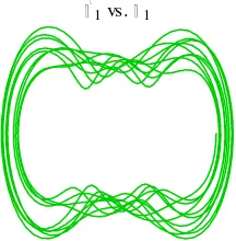
Gambar C.16, Ruang fasa dengan l

1

= 1-1.5

, θ

2

= 1.31

, dan θ

3

= 1.17

1vs. 1

1vs. 1

1vs. 1

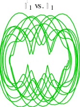
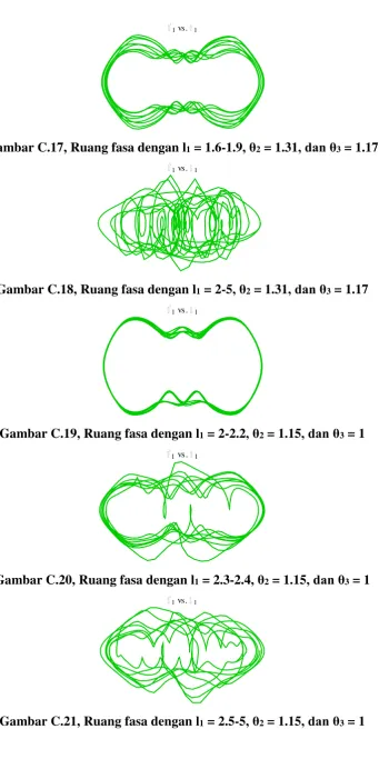
Gambar C.17, Ruang fasa dengan l

1

= 1.6-1.9

, θ

2

= 1.31

, dan θ

3

= 1.17

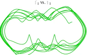
Gambar C.18, Ruang fasa dengan l

1

= 2-5

, θ

2

= 1.31

, dan θ

3

= 1.17

Gambar C.19, Ruang fasa dengan l

1

= 2-2.2

, θ

2

= 1.15

, dan θ

3

= 1

Gambar C.20, Ruang fasa dengan l

1

= 2.3-2.4

, θ

2

= 1.15

, dan θ

3

= 1

Gambar C.21, Ruang fasa dengan l

1

= 2.5-5

, θ

2

= 1.15

, dan θ

3

= 1

1vs. 1

1vs. 1

1vs. 1

1vs. 1

Gambar C.22, Ruang fasa dengan l

1

= 2.5-3

, θ

2

= 0.98

, dan θ

3

= 0.98

Gambar C.23, Ruang fasa dengan l

1

= 3.1-5,

θ

2

= 0.98

, dan θ

3

= 0.98



Grafik diagram fasa untuk Tabel 4.3 (Hasil pengujian keadaan sistem untuk variasi

panjang tali pendulum2, m

1

= m

2

= m

3

=1, l

1

= l

3

= 1, dan

θ

1

= Pi/2)

Gambar C.24, Ruang fasa dengan l

2

= 2,

θ

2

= 0-1.57

, dan θ

3

= 0-1.57



Grafik diagram fasa untuk Tabel 4.4 (Hasil pengujian keadaan sistem untuk variasi

panjang tali pendulum3, m

1

= m

2

= m

3

=1, l

1

= l

2

= 1, dan

θ

1

= Pi/2)

Gambar C.25, Ruang fasa dengan l

3

= 1.1-1.2,

θ

2

= 1.31

, dan θ

3

= 1.17

1vs. 1

1vs. 1

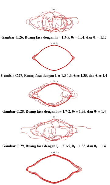
Gambar C.26, Ruang fasa dengan l

3

= 1.3-5,

θ

2

= 1.31

, dan θ

3

= 1.17

Gambar C.27, Ruang fasa dengan l

3

= 1.3-1.6,

θ

2

= 1.35

, dan θ

3

= 1.4

Gambar C.28, Ruang fasa dengan l

3

= 1.7-2,

θ

2

= 1.35

, dan θ

3

= 1.4

Gambar C.29, Ruang fasa dengan l

3

= 2.1-5,

θ

2

= 1.35

, dan θ

3

= 1.4

Gambar C.30, Ruang fasa dengan l

3

= 2.1-2.8,

θ

2

= 1.15

, dan θ

3

= 1.57

3vs. 3

3vs. 3

3vs. 3

3vs. 3

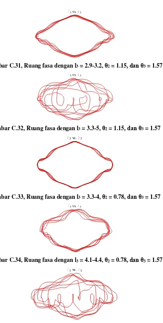
Gambar C.31, Ruang fasa dengan l

3

= 2.9-3.2,

θ

2

= 1.15

, dan θ

3

= 1.57

Gambar C.32, Ruang fasa dengan l

3

= 3.3-5,

θ

2

= 1.15

, dan θ

3

= 1.57

Gambar C.33, Ruang fasa dengan l

3

= 3.3-4,

θ

2

= 0.78,

dan θ

3

= 1.57

Gambar C.34, Ruang fasa dengan l

3

= 4.1-4.4,

θ

2

= 0.78

, dan θ

3

= 1.57

Gambar C.35, Ruang fasa dengan l

3

= 4.5-5,

θ

2

= 0.78

, dan θ

3

= 1.57

3vs. 3

3vs. 3

3vs. 3

3vs. 3



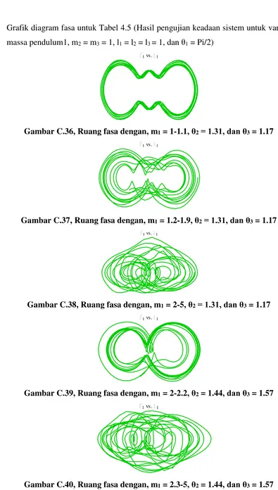
Grafik diagram fasa untuk Tabel 4.5 (Hasil pengujian keadaan sistem untuk variasi

massa pendulum1, m

2

= m

3

= 1, l

1

= l

2

= l

3

= 1, dan

θ

1

= Pi/2)

Gambar C.36, Ruang fasa dengan, m

1

= 1-1.1

, θ

2

= 1.31, dan θ

3

= 1.17

Gambar C.37, Ruang fasa dengan, m

1

= 1.2-1.9

, θ

2

= 1.31, dan θ

3

= 1.17

Gambar C.38, Ruang fasa dengan, m

1

= 2-5

, θ

2

= 1.31, dan θ

3

= 1.17

Gambar C.39, Ruang fasa dengan, m

1

= 2-2.2

, θ

2

= 1.44

, dan θ

3

= 1.57

Gambar C.40, Ruang fasa dengan, m

1

= 2.3-5

, θ

2

= 1.44

, dan θ

3

= 1.57

1vs. 1

1vs. 1

1vs. 1

1vs. 1



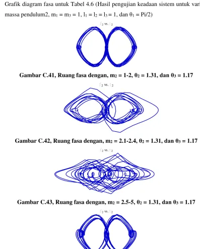
Grafik diagram fasa untuk Tabel 4.6 (Hasil pengujian keadaan sistem untuk variasi

massa pendulum2, m

1

= m

3

= 1, l

1

= l

2

= l

3

= 1, dan

θ

1

= Pi/2)

Gambar C.41, Ruang fasa dengan, m

2

= 1-2

, θ

2

= 1.31

, dan θ

3

= 1.17

Gambar C.42, Ruang fasa dengan, m

2

= 2.1-2.4

, θ

2

= 1.31

, dan θ

3

= 1.17

Gambar C.43, Ruang fasa dengan, m

2

= 2.5-5

, θ

2

= 1.31

, dan θ

3

= 1.17

Gambar C.44, Ruang fasa dengan, m

2

= 3

, θ

2

= 1.17

, dan θ

3

= 1

Gambar C.45, Ruang fasa dengan, m

2

= 3.1-5

, θ

2

= 1.17

, dan θ

3

= 1

2vs. 2

2vs. 2

2vs. 2

2vs. 2



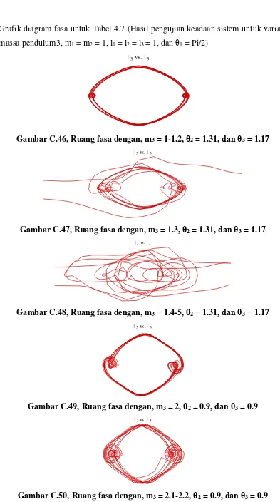
Grafik diagram fasa untuk Tabel 4.7 (Hasil pengujian keadaan sistem untuk variasi

massa pendulum3, m

1

= m

2

= 1, l

1

= l

2

= l

3

= 1, dan

θ

1

= Pi/2)

Gambar C.46, Ruang fasa dengan, m

3

= 1-1.2

, θ

2

= 1.31

, dan θ

3

= 1.17

Gambar C.47, Ruang fasa dengan, m

3

= 1.3

, θ

2

= 1.31

, dan θ

3

= 1.17

Gambar C.48, Ruang fasa dengan, m

3

= 1.4-5

, θ

2

= 1.31

, dan θ

3

= 1.17

Gambar C.49, Ruang fasa dengan, m

3

= 2

, θ

2

= 0.9

, dan θ

3

= 0.9

Gambar C.50, Ruang fasa dengan, m

3

= 2.1-2.2

, θ

2

= 0.9

, dan θ

3

= 0.9

3vs. 3

3vs. 3

3vs. 3

3vs. 3

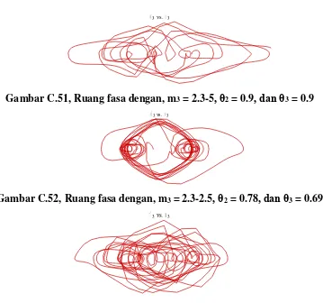
Gambar C.51, Ruang fasa dengan, m

3

= 2.3-5

, θ

2

= 0.9

, dan θ

3

= 0.9

Gambar C.52, Ruang fasa dengan, m

3

= 2.3-2.5

, θ

2

= 0.78

, dan θ

3

= 0.69

Gambar C.53, Ruang fasa dengan, m

3

= 2.6-5

, θ

2

= 0.78

, dan θ

3

= 0.69



Grafik diagram fasa untuk Tabel 4.8 (Hasil pengujian sistem untuk massa dan tali

yang sama)

Gambar C.54, Ruang fasa dengan m

1

= m

2

= m

3

= 2, l

1

= l

2

= l

3

= 1, θ

1

=

1.15-1.57, θ

2

= 1.31, dan

θ

3

= 1.17

Gambar C.55, Ruang fasa dengan m

1

= m

2

= m

3

= 3, l

1

= l

2

= l

3

= 1, θ

1

=

1.15-1.57, θ

2

= 1.31, dan θ

3

= 1.17

3vs. 3

3vs. 3

3vs. 3

1vs. 1

Gambar C.56, Ruang fasa dengan m

1

= m

2

= m

3

= 1, l

1

= l

2

= l

3

= 2

, θ

1

=

1.15-1.57, θ

2

= 1.31, dan θ

3

= 1.17

Gambar C.57, Ruang fasa dengan m

1

= m

2

= m

3

= 1, l

1

= l

2

= l

3

= 3

, θ

1

=

1.15-1.57, θ

2

= 1.31, dan θ

3

= 1.17

Gambar C.58, Ruang fasa dengan m

1

= m

2

= m

3

= l

1

= l

2

= l

3

= 2

, θ

1

= 1.15-1.57,

θ

2

= 1.31, dan θ

3

= 1.17

1vs. 1

1vs. 1