Dynamic evolution control for synchronous buck DC–DC
converter: Theory, model and simulation
Ahmad Saudi Samosir
a,b,*, Abdul Halim Mohd Yatim
ba
Universitas Lampung, Jl. Soemantri Brojonegoro No.1, Bandar Lampung 35145, Indonesia b
Universiti Teknologi Malaysia, UTM Skudai, 81310 Johor Bahru, Malaysia
a r t i c l e
i n f o
Article history: Received 24 April 2009
Received in revised form 1 January 2010 Accepted 11 January 2010
This paper proposes a new control technique for synchronous buck DC–DC converter. The-ory, design and implementation of the proposed control technique are provided. A new approach for converter controller synthesis based on dynamic evolution control theory is presented. In order to synthesize the converter controller, this method uses a simple anal-ysis of nonlinear equation models of the converter. The synthesis process is simple and requires a quite low bandwidth for the controller. Therefore, this control method is suitable for digital control implementation. As an illustrative example, the synthesis of synchronous buck DC–DC converter controller is discussed in detail. The model of the synchronous buck DC–DC converter system was implemented using SimPowerSystems toolbox of MATLAB-SIMULINK. Performance of the proposed dynamic evolution control under step load change and step input voltage condition was investigated. Simulation results confirm that the pro-posed control method is superior to traditional PI based controller because of fast transient response and good disturbance rejection.
Ó2010 Elsevier B.V. All rights reserved.
1. Introduction
According to the growth of power electronics application, the use of the synchronous buck converter has increased. This converter is one of the most common converter topologies that are usually used in power electronics application[2,12]. Syn-chronous buck converters are step-down switching-mode power converters. They are popular because of their high effi-ciency and compact size. They are used in place of linear voltage regulators at a relatively high output power. Synchronous buck converters are the most widely used type of power converter in battery-powered applications. Many application of power electronics converter use the synchronous buck converter as their basic topology. For example, syn-chronous buck converter is usually used in high efficiency power supplies.
In view of this, the need of good controllers for synchronous buck converter also increases. There is an increasing need for good controllers to obtain precise output voltage regulation under different supply and load conditions.
Synchronous buck converters represent a challenging field for sophisticated control techniques application due to their intrinsic nature of nonlinear and time-variant systems[11–15]. In terms of converter controller design, the use of averaging or sampling techniques, followed by linearization and small-signal analysis allows the derivation of linear time-invariant dynamic models for any converter topology. This approach enables the designer to use a simple linear controller to keep the system stable. However, they are normally dependent on the converter’s operating point[4–8]. In other words, it is only
1569-190X/$ - see front matterÓ2010 Elsevier B.V. All rights reserved.
doi:10.1016/j.simpat.2010.01.010
*Corresponding author. Address: Universiti Teknologi Malaysia, UTM Skudai, 81310 Johor Bahru, Malaysia. Tel.: +60 7 5535829.
applicable for a near specified operating point, while the parameters of any transfer function or state-space matrix describing a DC–DC converter may vary depending on its output voltage, input voltage or load current.
In this paper, a new approach for synchronous buck converter controller’s synthesis based on dynamic evolution control theory is presented. The proposed dynamic evolution control exploits the non-linearity and time-varying properties of the system to make it a superior controller. This control method tries to overcome the mentioned problem of linear control by explicitly using dynamic equation model of the converter for control synthesis. Synthesis example of dynamic evolution con-trol, when applied to synchronous buck DC–DC converter, is discussed in detail. In order to synthesize the converter control-lers, this method uses a simple analysis of nonlinear equation models of the converter.
This paper explores the potential and feasibility of dynamic evolution control for power electronics circuits. Synchronous buck converter is considered to exhibit that satisfactory voltage regulation can be achieved without having to obtain com-plex mathematical models for large signals or having to estimate the range of parameter variation.
The synthesis process is simple and requires a low bandwidth for the controller. Therefore it only requires simple calcu-lations and easy to realize in digital format, thus suitable for digital control implementation.
A comprehensive simulation analysis was conducted to verify the controller performance. The performance of dynamic evolution control under step load variation condition is tested through simulation by using Matlab-Simulink. Simulation re-sults are presented to explore the potentials of dynamic evolution control for applications to power electronics circuits.
The results shown that dynamic evolution control is expected to obtain several advantages such as zero steady-state er-ror, wide range stability, and robust performance. Moreover, the dynamic evolution control is operated at constant switching frequency. Hence, the problems of power filtering are reduced.
2. Dynamic evolution control
The dynamic evolution control (DEC) is derived based on the basic terminology of control theory, especially the definition of feedback control. Definition states, ‘feedback control refers to an operation that, in the presence of disturbances, tends to reduce the difference between the output of a system and some reference input and that does so on the basis of this differ-ence’[1].
From this definition we make the assumption that, ‘‘The difference between output and the reference input in a controlled system, denotes as the error state, must be reduced to zero at any instant of time, regardless, whether the disturbance is present or not”.
In connection with this assumption, the DEC proposes a technique to control the dynamic evolution of the error state of the controlled system. In dynamic evolution control, the error state is forced to go to zero by following a specific path, called the evolution path. This evolution path ensures the error state must be reduced toward zero at the increase of time.
Design of the DEC-based controller[3,9,10]can be described as follows:
1. Evolution path selection. 2. Dynamic evolution function. 3. Analysis of converter system. 4. Synthesis of duty cycle formula. 5. PWM duty cycle generation.
2.1. Evolution path
The first step that needs to be done in the DEC-based control design is to determine the evolution path that ensures the error state will go to zero at any instant of time. In an effort to determine the evolution path, we have plot the evolution path based on an approach to the dynamic response of second order system.
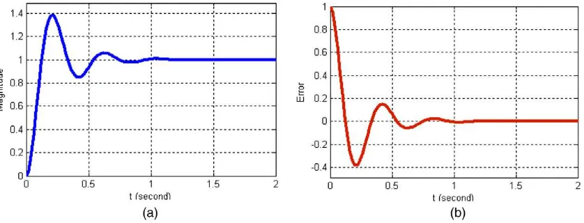
Fig. 1a shows the dynamic response of second order system in time domain. This figure shows that, in the increase of time, the magnitude of system output should lead to a value determined by a reference input. A common observation in sec-ond order system is that an overshoot and oscillations are inherent on the magnitude of system output.
By analyzing the error state of this second order system, the dynamic evolution of error state can be depicted as inFig. 1b. From this figure, it can be considered that the magnitude of error will decrease to zero in the increase of time. Similarly as in the magnitude of system output, an ‘overshoot’ and oscillations are present on the evolution of magnitude of error.
An approach to improve the performance of the system is done by controlling the output response of the system so that no overshoot and oscillations occurs as shown inFig. 2a. The figure shows for an ideal output response, the magnitude of system output from zero origin increases to a value determined by a set reference input and maintains this value upon reach-ing this state.
In terms of the error, the ideal error trajectory is as shown inFig. 2b. With the initial error is positive, the magnitude of error will decrease to zero in the increase of time and maintains this position.
2.1.1. Piecewise linear evolution path
As the first approximation, the ideal error trajectory fromFig. 2b is approximated as two straight lines. The first line de-scribes the movement of the error from positive values to zero. This line shows that when the initial value of error is positive, in the increase of time, the value of error must decrease towards zero. The second line describes the movement of the error after reaching the zero position. This line shows that when the error has reached zero, it will maintain this position over time.
Since the initial values of the error can be either be positive or negative, a third line must be added to accommodate the movement of error from negative values goes to zero. This line shows that when the initial value of error is negative, in the increase of time, the value of error must increase towards zero.
Hence, the evolution path of error state can be drawn as a piecewise linear graph as inFig. 3. When the initial value of error is positive, the error is decreased to zero in accordance to lineY1. After reaching zero position, the error will maintain in
the zero position in accordance to lineY0. On the other hand, if the initial value of error is negative, the error is increased to
zero in accordance to lineY2.
FromFig. 3, the equation of linesY0,Y1, andY2can be written as:
Y0¼0 ð1Þ
Y1¼Cm:t ð2Þ
Y2¼ Cþm:t ð3Þ
whereCis the initial value ofY, andmis proportional to the slope ofY1.
InFig. 3, if the initial value ofYis positive, the value ofYdecrease linearly to zero as a function of time by followingY1, on
the other hand if the initial value ofYis negative, the absolute value ofYincrease linearly to zero as a function of time by followingY2. The steepness of the slope ofY1is proportional to the slope factor m and when the value ofYreaches the zero
position (Y= 0), it maintains this position atY0condition.
Fig. 1.(a) Dynamic response of second order system. (b) Error.
In general form, the equation ofY0,Y1, andY2from(1)–(3), can be represented as:
Y¼ ðCm:tÞ:u ð4Þ
whereuis the specific coefficient ofYand the value ofuis given as:
u¼
1; for Y<0 0; for Y¼0
þ1; for Y>0
8
> <
> :
9
> =
> ;
ð5Þ
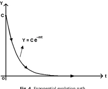
2.1.2. Exponential evolution path
For the second approximation, the ideal error trajectory shown inFig. 2b is approximated as an exponential function as shown inFig. 4. The concept is the same as described in A except that the trajectory function is exponential instead of straight lines. The equation of this trajectory is given in(6). With this approximation, the equation of the evolution path is unique. This equation applies to both initial values of positive or negative. Even though the initial values of error are po-sitive or negative the error state move to zero position by following this equation.
Y¼Cemt ð6Þ
whereCis the initial value ofY, andmis proportional to the initial decrease rate ofY.
2.2. Dynamic evolution function
The objective of the dynamic evolution control is to control the dynamic characteristic of the system and operate on the target equation,Y= 0. In the dynamic evolution control system, the dynamic characteristics of converter system are forced to follow an evolution path. This evolution path must decrease to zero accordingly with time. In this paper, the selected evo-lution path is an exponential function as shown inFig. 4. With this exponential function, the value ofYis decrease exponen-tially to zero as a function of time. The decrease slope ofYis proportional to the decrease ratem.
Fig. 3.Piecewise linear evolution path.
IfYrepresents the state errors function of the converter, andYis forced to follow the evolution path as show inFig. 4, so the dynamic evolution of the error state function (Y), with initial valueY0, can be represented as
Y¼Yo:emt ð7Þ
It means that the error state function (Y) is forcely decreased to zero exponentially with a decrease ratem. From(7), the derivative ofYis given as:
dY
dt ¼ m:Yo:e
mt
Hence,
dY
dt ¼ m:Y
As a result, the dynamic evolution function can be written as Eq.(8).
dY
dtþmY¼0; m>0 ð8Þ
where,mis a design parameter specifying the rate of evolution.
The dynamic evolution function(8)will drive the error state function (Y) of system, decrease to zero exponentially with the decrease rate m.
2.3. Analysis of converter system
The objective of the converter system analysis is to obtain the equation of converter output response. This equation will be used for formulating the duty cycle function in the synthesis process.
2.4. Synthesis process
The main objective of the synthesis process is to obtain the control law that guarantees the error state function (Y) of sys-tem decrease to zero by following the evolution path. In DC–DC power converters, this control law represents the duty cycle equation of the converter. This duty cycle equation
a
(v
O,Vg,iL), representsa
as a function of the statev
O,Vg, andiL.In order to obtain the duty cycle equation
a
(v
O,Vg,iL), the dynamic equation of the converter system is analyzed andsubstituted into the dynamic evolution function(8).
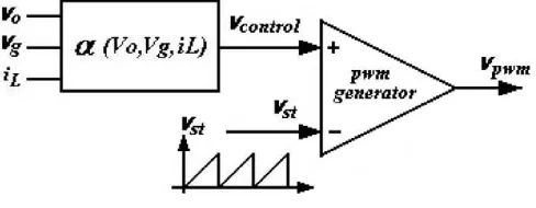
2.5. PWM duty cycle generation
The duty cycle equation is used to calculate the desired value of signal level control
v
control. The pwm signal is generatedby comparing a signal level control
v
controlwith a repetitive waveform as shown inFig. 5. The frequency of the repetitivewaveform with a constant peak, which is a sawtooth
v
st, establishes the switching frequency. This frequency is kept constant.Therefore, the dynamic evolution control is operated at constant switching frequency.
3. Model of synchronous buck DC–DC converter
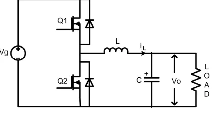
The synchronous buck converter is essentially the same as the buck step-down converter with the substitution of the diode for another FET switch. The top FET switch behaves the same way as the buck converter in charging the inductor cur-rent. When the switch control is off, the lower FET switch turns onto provide a current path for the inductor when discharg-ing. Although requiring more components and additional switch logic sequencing, this topology improves efficiency with faster switch turn-on time and lower FET series resistance (rdson) versus the diode.
A schematic diagram for the synchronous buck DC–DC converter is shown inFig. 6. The state-space averaged model describing the voltage and current dynamics of the synchronous DC–DC buck converter are given by
LdiLðtÞ
whereLis the inductance,Cthe capacitance,Rthe loading resistance,Vg(t) the input voltage,iL(t) the inductor current,
v
O(t) the output voltage anda
(t) the duty cycle, respectively.Rearranging(4), the output voltage of converter can be written as:
v
OðtÞ ¼VgðtÞ:a
ðtÞ LdiLðtÞdt ð11Þ
4. Synthesis of synchronous buck converter controller
Synchronous buck converter inFig. 6has two FET switches. Because of those FET switches are operated in complemen-tary, it is sufficient to determine the control function of the top switch only.
The dynamic evolution synthesis of the controller begins by defining the state error function (Y). In power electronics application,Ycan be selected as a function of error voltage or error current. In this paper, the selectedYis a linear function of error voltage as
Y¼k:
v
errðtÞ ð12Þwherekis a positive coefficient, and
v
erris error voltage:v
errðtÞ ¼Vrefv
OðtÞ ð13ÞThe derivative ofYis given by:
dY
dt ¼k
d
v
errðtÞdt ð14Þ
Substituting(12) and (14)into(8), yields
kd
v
errðtÞdt þm:k:
v
errðtÞ ¼0 ð15ÞDirectly summing the state operating point of converter(11)into(15)we can get:
kd
v
errðtÞdt þm:k:
v
errðtÞ þv
OðtÞ ¼VgðtÞ:a
ðtÞ L diLðtÞdt ð16Þ
Solving for
a
, the obtained duty cycle equationa
ðtÞis given by:a
ðtÞ ¼kwhere the expression for duty cycle
a
ðtÞis the control action of the converter controller.Duty cycle Eq.(17)forces the state error function (Y) to satisfy the dynamic evolution function(8). Consequently, in the increase of time, the state error function (Y) is forced to make evolution by following Eq.(7)and decrease to zero (Y= 0) with a decrease rate m. Therefore, in the steady-state condition, the state error function (Y) satisfy the equation
Y¼k:
v
errðt¼Þ ¼0Thus the state error of the converter will converge to zero.
v
errðt¼Þ ¼0 ð18ÞSubstituting(13)into(18), we can see that the voltage output of converter converges to the converter’s steady-state:
v
Oðt¼Þ ¼Vref ð19ÞFrom the synthesis procedure, it is clear that the dynamic evolution controller works well for nonlinear systems and does not need any linearization or simplification on the system model at all, as normally required in conventional control techniques.
Rearranging the duty cycle Eq.(17), the control function can be written as:
a
ðtÞ ¼ VrefVgðtÞþ
ðmk1Þ
VgðtÞ
v
errðtÞ þ kVgðtÞ d
v
errðtÞdt þ
L VgðtÞ
diLðtÞ
dt ð20Þ
It is interesting to note that the control function in(20)consists of four distinct parts. The first part is the feedforward term, Vref
VgðtÞ, which is calculated based on the duty cycle at the previous sampling instant. This term compensates for variations in the input voltages.
The second and third terms are similar to the proportional and derivative terms of the perturbations in the output voltage respectively. But the important feature that makes this controller better than the conventional one is that the gain value of the proportional and derivative terms are not fixed. This gain varies with the input voltage. The last term consists of the derivative terms of the inductor current. The gain of this term is also varying with the input voltage.
From(20), we can see that the input voltage, output voltage and inductor current influence in control output. The advan-tage is the dynamic evolution control can compensate the variations in the input and output voladvan-tages and the change of inductor current. It contributes to a better dynamic performance of the controlled system.
For design of a digital dynamic evolution controller, the continuous-time duty cycle Eq.(17)can be transformed to a
dis-5.1. Validation of dynamic evolution control theory
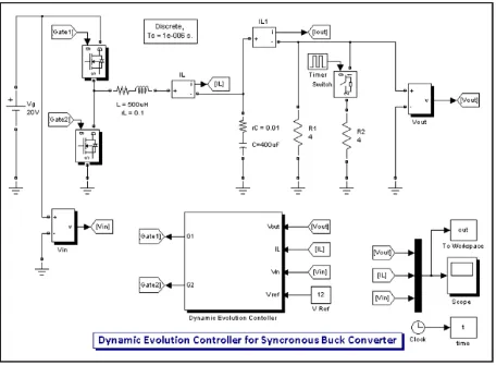
In order to verify the working concept of dynamic evolution control, a comprehensive simulation analysis was conducted. The simulations were performed in Matlab-Simulink environment. The synchronous buck converter scheme and the dy-namic evolution control law, which is described by(17), are modelled in Simulink as shown inFig. 7. The model parameters are listed inTable 1.
Investigation begins by studying the time response of output voltage of synchronous buck DC–DC converter which is con-trolled with dynamic evolution control. Input voltage is set to 20 V. The reference output voltage was change from 0 to 12 V att= 0. Controller parameter was set tok= 0.1. Time response is investigated for different gain m values within ranges from 500 to 6000.
Fig. 8shows the simulation result of the converter time response with various values of gain m. From the simulation re-sult, we can see that when the value of gain m is low, the response of converter is slow. When the value of gain m is higher, response of converter is faster. It is mean that, the higher value of gain m gives a faster response of controller. The overshoot will occur on the converter output voltage when the value of gain m is very high. Therefore, the best m value is the maximum value of gain m before the overshoot appears.
Fig. 9shows the error voltage of converter with respect to different values of gainm. This result shows that the error volt-age decrease to zero exponentially at a decrease rate depending on the value of gainm. Largemvalues make the error voltage goes to zero faster. The trajectories of converter with different values of gainmare shown inFig. 10.
Table 1
0 0.001 0.002 0.003 0.004 0.005 0.006 0.007 0.008 0.009 0.01 0
5.2. Investigation of controller performance
To test the performance of the proposed controller, a comprehensive simulation under step load change with constant and varying input voltage were tested. The reference output voltage was set to 12 V and the load demand was set between 3A and 6A every 20 ms. Depending on the simulation result in Fig. 8, the controller parameters are set to k= 0.1 and
m= 3000.
Here the situation where the load changes suddenly from one value of load resistance to another is considered. This is particularly interesting because it is a typical problem for power electronics, where the power supply is supposed to com-pensate quickly for the load variation.
Figs. 11 and 12show the performance of the proposed controller under step load change condition.Fig. 11shows the sim-ulation result under step load change with constant input voltage. The input voltage was fixed to 20 V. At time 20 ms, a step load change occurs, the load resistance changes from 4 to 2O. As a result of this change, it is shown that the inductor current changes from 3A to 6A. The drop in the regulated output voltage went down by 0.5 V and it took about 2 ms for it to settle down at 21 V. From this result we can say that the controllers accomplish to regulate the converter output voltage at a stea-dy-state voltage of 12 V reference.
0 0.001 0.002 0.003 0.004 0.005 0.006 0.007 0.008 0.009 0.01 -2
Fig. 9.Error voltage of synchronous buck converter with differentm.
-2 0 2 4 6 8 10 12
Trajectory of dynamic evolution control with difference m
m=6000
Fig. 12shows the simulation result under step load change with varying input voltage. Input voltage was set to varying voltage, of a 20 Vdcvoltage with an addition of a 5 V, 100 Hz ripple voltage. The same disturbance setting was applied. At time 20 ms, the load resistance was change from 4 to 2O. As a result, the inductor current was suddenly changed from 3A to 6A. The drop on the regulated output voltage went down to 0.5 V and it took around 2 ms to settle down. This result is sim-ilar to the result inFig. 11. It means that the controller completely reduced the effect of the ripple disturbance in the input voltage. Clearly, the proposed controller is able to perform satisfactorily well with excellent disturbance rejection and fast response.
6. Controller performance comparison
In order to compare the performance of the proposed controller to other control methods, a Simulink model of the buck converter scheme was designed as a plant. According to the experimental result that have been reported in Ref.[14], the Simulink model of DC–DC buck converter has been created withL= 1 mH, C= 120
l
F, nominal input voltageVg= 50 V. The nominal load current was 1A. The output regulated voltage was set to 10 V and the nominal loading resistorRwas 10O. The buck converter parameters are listed inTable 2. The same disturbance with step load change and step input voltage0 0.01 0.02 0.03 0.04 0.05 0.06 0.07 0.08 0.09 0.1
Fig. 11.Simulation result under step load change with constant input voltage.
0 0.01 0.02 0.03 0.04 0.05 0.06 0.07 0.08 0.09 0.1
change were tested to the conventional single-loop PI, double-loop PI controller and the proposed dynamic evolution control.
Three kinds of controller were applied to the same plant. The first one is a conventional single-loop PI. As in[14], the transfer function for the single-loop PI controller was given by
GPIðsÞ ¼0:0001þ1
Fig. 13.Performance of single-loop PI controller under step load change.
0.26 0.27 0.28 0.29 0.3 0.31 0.32 0.33 0.34
The single-loop PI controller was obtained in such a way that the closed-loop step response under nominal working con-ditions did not have any overshoots and the closed-loop system was well damped even under light load concon-ditions[14].
The second controller method was the cascade controller or double-loop PI controller. Referring to[14], for the voltage loop, the controller parameter was set to
GPI1ðsÞ ¼0:1þ
The third controller method is the proposed dynamic evolution control. With reference to the simulation result inFig. 5, the controller parameters was set tok= 0.1 andm= 3000.
6.1. Load-regulation performance
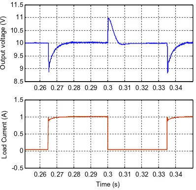
The reference output voltage was set to 10 V and the load demand was switched between 1A and 0.01A by changing the loading resistor with a MOSFET which was driven by a square-wave signal generator.Fig. 13shows the performance of
0.26 0.27 0.28 0.29 0.3 0.31 0.32 0.33 0.34
Fig. 15.Performance of dynamic evolution controller under step load change.
0.4 0.6 0.8 1 1.2
output voltage and load current of the conventional single-loop PI controller. The drop voltage on the regulated output went down as high as 5 V and it took more than 100 ms to settle down.Fig. 14shows the performance of output voltage and load current of the double-loop PI controller with the same load demand. The drop voltage on the regulated output decreased to 1 V and it took around 10 ms to settle down.Fig. 15shows the performance of output voltage and load current of the pro-posed controller with the same load demand. The drop voltage on the regulated output decreased to less than 0.5 V, and it took around 2 ms to settle down.
Clearly, the performance of the dynamic evolution controller was far superior to the conventional single-loop and double-loop PI controller having better disturbance rejection and faster response.
6.2. Input voltage regulation performance
The reference output voltage was set to 10 V with constant current demand of 1A. However the supply voltage was switched between 27 and 50 V.Fig. 16shows the performance of output voltage of the conventional single-loop PI controller when the input voltage was changed. The drop voltage on the regulated output went as high as 10 V when the supply voltage was changed from 27 to 50 V and it took around 50 ms for the output to settle down.Fig. 17shows the performance of the double-loop PI controller with the same change in supply. The drop voltage on the regulated output went down to 1 V when
0.1 0.12 0.14 0.16 0.18 0.2
8
0.1 0.12 0.14 0.16 0.18 0.2
20 40 60
Time (s)
Input Voltage (V)
Fig. 17.Performance of double-loop PI controller under step input voltage change.
the supply voltage was changed from 27 to 50 V and it took around 10 ms to settle down.Fig. 18shows the performance of the proposed controller with the same changing supply. The drop voltage on the regulated output went down to less than 0.1 V when the supply voltage was changed from 27 to 50 V and it took around 5 ms to settle down.
Again, the dynamic evolution controller outperformed the conventional single-loop and double-loop PI controller having better disturbance rejection and a faster response.
7. Conclusions
A new control technique has been presented and implemented successfully for the controller of a synchronous buck DC–DC converter. The performance of dynamic evolution control under step load change and step input voltage change con-dition has been tested and compared with single-loop and double-loop PI controller. From the result, the proposed dynamic evolution controller outperforms a conventional single-loop and double-loop PI controller with better disturbance rejection and a faster response. The controller has been shown to be robust against load changes and supply changes.
The advantages of the proposed dynamic evolution control controller compared with the conventional PID controller are:
DEC has just one parameter that must be tuned, instead of the PID which have two or three parameters. In the case of double-loop PID, there are 4 or 5 parameters making it easier to tune.
Good response to the variations of input and output voltage. Fast response and stable.
However the disadvantage of DEC is that the duty cycle calculation has a division component, making it difficult to imple-ment in analog circuit form.
References
[1] K. Ogata, Modern Control Engineering, Prentice-Hall, Inc., 1997.
[2] A.R. Oliva, S.S. Ang, G.E. Bortolotto, Digital control of a voltage-mode synchronous buck converter, IEEE Transactions on Power Electronics (January) (2006) 157–163.
[3] A.S. Samosir, A.H.M. Yatim, Implementation of new control method based on dynamic evolution control for DC–DC power converter, International Review of Electrical Engineering Journal (February) (2009) 1–6.
[4] S.C. Tan, Y.M. Lai, C.K. Tse, M.K.H. Cheung, A fixed-frequency pulse-width-modulation based quasi sliding mode controller for buck converters, IEEE Transactions on Power Electron. (November) (2005) 1379–1392.
[5] S.C. Tan, Y.M. Lai, C.K. Tse, M.K.H. Cheung, Adaptive feedforward and feedback control schemes for sliding mode controlled power converters, IEEE Transactions on Power Electronics (January) (2006) 182–192.
[6] T. Chang, D. Yuan, H. Hanek, Matched feedforward/model reference control of a high precision robot with dead-zone, IEEE Transactions on Control System Technology (January) (2008) 94–102.
[7] V.S.C. Raviraj, P.C. Sen, Comparative study of proportional–integral, sliding mode, and fuzzy logic controllers for power converters, IEEE Transactions on Industry Applications (March) (1997) 518–524.
[8] A. Kolesnikov, G. Veselov, A. Kolesnikov, A. Monti, F. Ponci, E. Santi, R. Dougal, Synergetic synthesis of DC–DC boost converter controllers: theory and experimental analysis, IEEE APEC (March) (2002) 409–415.
[9] A.S. Samosir, A.H.M. Yatim, Implementation of new control method based on dynamic evolution control with linear evolution path for boost DC–DC converter, PECON (December) (2008) 213–218.
[10] A.S. Samosir, A.H.M. Yatim, Dynamic evolution control of bidirectional DC–DC converter for interfacing ultracapacitor energy storage to fuel cell electric vehicle system, AUPEC (December) (2008) 1–6.
[11] H. Erdem, Comparison of fuzzy, PI and fixed frequency sliding mode controller for DC–DC converters, ACEM (September) (2007) 684–689. [12] S. Uran, M. Milanovic, State controller for buck converter, in: Proceedings of the IEEE Region 8 Conference on Computer as a Tool, EUROCON, vol. 1,
2003, pp. 381–385.