CHAPTER IV RESULT OF THE STUDY
In this chapter, the writer presented the data which had been collected from the research in the field of study. The data are the result of pre test score in essay test of experimental class, the result of pre-test score in multiple choices test of experimental class, the result of post test score in essay test of experimental class, the result of post-test in multiple choices test of experimental class, result of data analysis, and discussion.
A. Description of the Data
In this chapter, the writer presented the obtaine data. The data are presented in the following steps.
1. The Result Pre Test Score of Essay Test of The Experiment Class
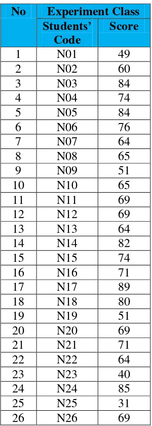
The writer gave pre test used essay test for the experimental class. It was conducted on Saturday, September 5th, 2015, at 09.45 – 11.05 am; in VII-1 room with the number of student were 26 students.
The scores of essay test are presented in the following table:
Table 4.1 The Result of Pre Test Score on Essay Test of Experimental Class No Experiment Class
Students’ Code
Score
1 N01 30
2 N02 47
3 N03 67
4 N04 60
5 N05 57
No Experiment Class
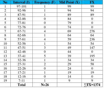
Based on the data above, it can be seen that the students’ highest score is 100 and the student’s lowest score is 7. To determine the range of score, the class interval, and interval of temporary, the writer calculated using formula as follows:
Interval of temporary (I) =R
K = 94
5 = 18.8 = 19
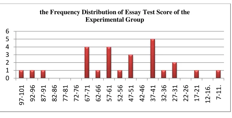
Figure 4.3 the Frequency Distribution of Essay Test Score of the Experimental Group
It can be seen from the figure above, the students’ pre-test scores in experimental group. There is one student who got score 97-100. There is one student who got score 92-96. There is one student who got score 87-91. There are four students who got score 67-71. There is one student who got score 62-66. There are four students who got score 57-61. There is one student who got score 52-56. There are three students who got score 47-51. There are five students who got score 37-41. There is one student who got score 32-36. There are two students who got score 231. There is one student who got score 121. There is one student who got score 7-11.
The next step, the writer tabulated the score of essay of experiment class into table for calculating of mean, median, and modus as follows:
0
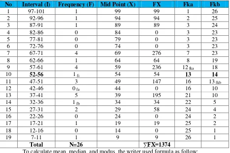
Table 4.4 The Calculation of Mean, Median, and Modus of Essay Test Score of the Experiment Class
No Interval (I) Frequency (F) Mid Point (X) FX Fka Fkb
fka: 12 i: 5
u: 56 + 0.5 = 56.5
𝑀𝑑𝑛 =𝑢 −
1
2𝑁 − 𝑓𝑘𝑎
𝑓𝑖 ×𝑖
= 56.5 − 1 2∙26−12
1 × 5
= 56.5 − 13−12
1 × 5
= 56.5 −1
1× 5
= 56.5 −5 = 51.5
c. Modus
Score: 52 – 56 fa: 0
fb: 1 i: 5
u: 56 + 0.5 = 56.5
𝑀𝑜 =𝑢 − 𝑓𝑏
𝑓𝑎+𝑓𝑏 ×𝑖
= 56.5− 1
0 + 1 × 5
= 56.5−1 1× 5
Based on the calculation above, it could be seen that mean of experiment class is 52.8, median was 51.5, and modus is 51.5.
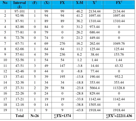
The last step, the writer tabulated the score of essay test of experiment class into table for calculating of standard deviation and standard error as follows:
Table 4.5 The Calculation of Standard Deviation and Standard Error of Essay Test Score of the Experiment Class
To calculate standard deviation and standard error, the writer used formula as follow:
d. Standard Deviation
𝑆𝐷 = ∑𝑓𝑥
2
𝑁
= 22211.436 26
= 854.286
= 29.228
e. Standard Error
𝑆𝑒𝑚 = 𝑠𝑑
𝑛 −1
= 29.228 26−1=
29.228
25 =
29.228
5 = 5.845
Based on the calculation above, it could be seen that standard deviation is 29.228 and standard error is 5.845.
2. The Result of Pre Test Score in Multiple Choices Test of the Experiment Class
The test scores of experimental group are presented in the following table. Table 4.6 The result of Pre Test Score on Multiple Choices Test of
Experimental Class No Experiment Class
Students’
The highest score (H) : 89 The lowest score (L) : 31
The range of score (R) = H−L + 1 = 89−31 + 1
= 58 + 1
= 59
Interval of temporary (I) =R
K = 59
6 = 9.83 = 10
From the calculation above, it could be seen that the range of score is 59 and interval of temporary is 6. Then, it is presented using frequency distribution in table 1.1 as follow:
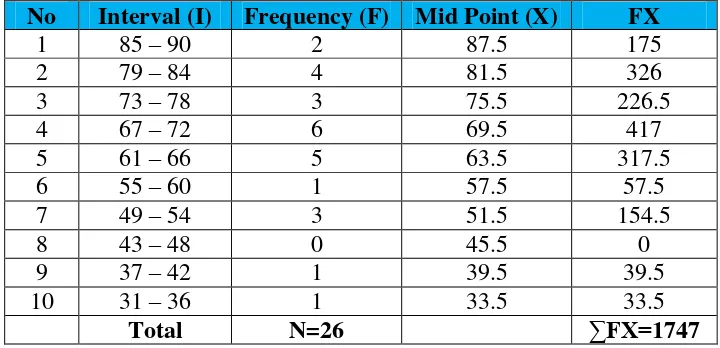
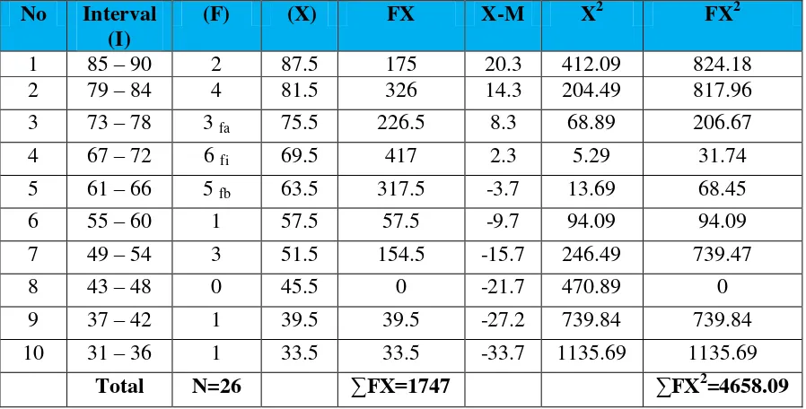
Table 4.7 Frequency Distribution of Pre Test Score in Multiple Choices Test of the Experiment Class
No Interval (I) Frequency (F) Mid Point (X) FX
1 85 – 90 2 87.5 175
2 79 – 84 4 81.5 326
3 73 – 78 3 75.5 226.5
4 67 – 72 6 69.5 417
5 61 – 66 5 63.5 317.5
6 55 – 60 1 57.5 57.5
7 49 – 54 3 51.5 154.5
8 43 – 48 0 45.5 0
9 37 – 42 1 39.5 39.5
10 31 – 36 1 33.5 33.5
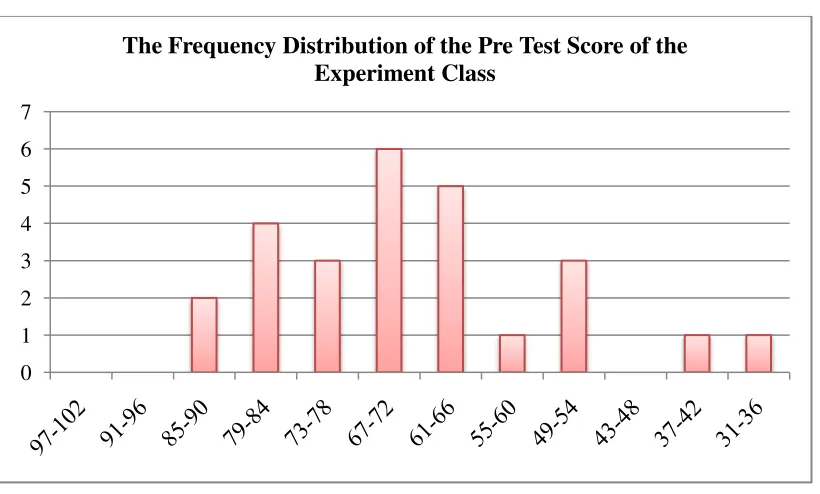
Figure 4.8 the Frequency Distribution of Pre-test Score in Multiple Choices Test of the Experimental Group
It can be seen from the figure above, the students’ pre-test scores in experimental group. There are two students who got score 85-90. There are four students who got score 79-84. There are three students who got score 73-78. There are six students who got score 67-72. There are five students who got score 61-66. There is one student who got score 55-60. There are three students who got score 49-54. There is one student who got score 37-42. There is one student who got score 31-36.
The next step, the writer tabulated the score of pre test of experiment class into table for calculating of mean, median, and modus as follows:
0 1 2 3 4 5 6 7
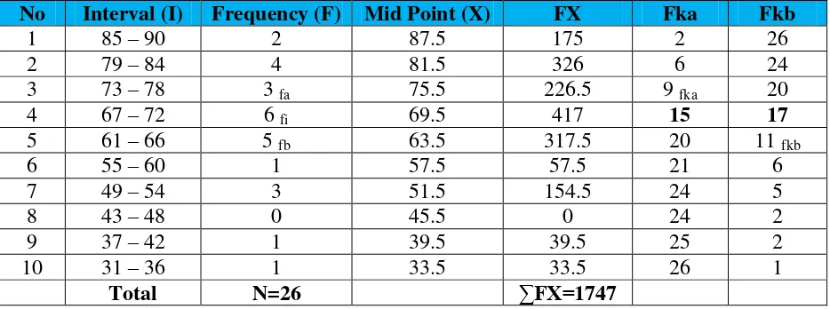
Table 4.9 The Calculation of Mean, Median, and Modus of Pre Test Score in Multiple Choices Test of the Experiment Class
No Interval (I) Frequency (F) Mid Point (X) FX Fka Fkb
1 85 – 90 2 87.5 175 2 26
2 79 – 84 4 81.5 326 6 24
3 73 – 78 3 fa 75.5 226.5 9 fka 20
4 67 – 72 6 fi 69.5 417 15 17
5 61 – 66 5 fb 63.5 317.5 20 11 fkb
6 55 – 60 1 57.5 57.5 21 6
7 49 – 54 3 51.5 154.5 24 5
8 43 – 48 0 45.5 0 24 2
9 37 – 42 1 39.5 39.5 25 2
10 31 – 36 1 33.5 33.5 26 1
Total N=26 ∑FX=1747
To calculate mean, median, and modus, the writer used formula as follow: a. Mean
𝑀𝑥 =∑𝑓𝑥
𝑁
=1747 26
= 67.2
b. Median Score: 67 – 72 fi: 6
fka: 9 i: 6
𝑀𝑑𝑛 =𝑢 − 1
2𝑁 − 𝑓𝑘𝑎
𝑓𝑖 ×𝑖
= 72.5 − 1 2∙26−9
6 × 6
= 72.5 − 13−9
6 × 6
= 72.5 −4
6× 6
= 72.5 −4 = 68.5
c. Modus
Score: 67 – 72 fa: 3
fb: 5 i: 6
u: 72 + 0.5 = 72.5
𝑀𝑜 =𝑢 − 𝑓𝑏
𝑓𝑎+𝑓𝑏 ×𝑖
= 72.5− 5
3 + 5 × 6
= 72.5−5 8× 6
= 72.5−3.75 = 68.75
The last step, the writer tabulated the score of pre test of experiment class into table for calculating of standard deviation and standard error as follows:
Table 4.10 The Calculation of Standard Deviation and Standard Error of Pre Test Score in Multiple Choices Test of the Experiment Class
No Interval (I)
(F) (X) FX X-M X2 FX2
1 85 – 90 2 87.5 175 20.3 412.09 824.18
2 79 – 84 4 81.5 326 14.3 204.49 817.96
3 73 – 78 3 fa 75.5 226.5 8.3 68.89 206.67
4 67 – 72 6 fi 69.5 417 2.3 5.29 31.74
5 61 – 66 5 fb 63.5 317.5 -3.7 13.69 68.45
6 55 – 60 1 57.5 57.5 -9.7 94.09 94.09
7 49 – 54 3 51.5 154.5 -15.7 246.49 739.47
8 43 – 48 0 45.5 0 -21.7 470.89 0
9 37 – 42 1 39.5 39.5 -27.2 739.84 739.84
10 31 – 36 1 33.5 33.5 -33.7 1135.69 1135.69
Total N=26 ∑FX=1747 ∑FX2=4658.09
To calculate standard deviation and standard error, the writer used formula as follow:
a. Standard Deviation
𝑆𝐷 = ∑𝑓𝑥
2
𝑁
= 4658.09 26
= 179.157
b. Standard Error 13.384 and standard error is 2.676.
3. The Result of Post Test Score in Essay Test of Experimental Class
The writer gave post test used essay test to the experiment class. First, post test was conducted to the experiment class. It was conducted on Saturday, Oktober 03th, 2015, at 07.15 – 08.35 am; in VII-1 room with the number of student were 26 students.
The scores of essay test are presented in the following table:
Table 4.11 The Result of Post Test Score in Essay Test of Experimental Class No Experiment Class
No Experiment Class
Based on the data above, it can be seen that the students’ highest score is 100 and the student’s lowest score is 18. To determine the range of score, the class interval, and interval of temporary, the writer calculated using formula as follows: The highest score (H) : 100
Interval of temporary (I) =R
K = 83
From the calculation above, it could be seen that the range of score is 83 and interval of temporary is 6. Then, it is presented using frequency distribution in table 1.1 as follow:
Table 4.12, Frequency Distribution of Essay Test Score of the Experiment Class
No Interval (I) Frequency (F) Mid Point (X)
FX
1 102-107 0 104.5 0
2 96-101 1 98.5 98.5
3 90-95 5 92.5 477.5
4 84-89 0 86.5 0
5 78-83 4 80.5 322
6 72-77 1 74.5 74.5
7 66-71 1 68.5 68.5
8 60-65 0 62.5 0
9 54-59 0 56.5 0
10 48-53 2 50.5 101
11 42-47 1 44.5 44.5
12 36-41 6 38.5 231
13 30-35 2 32.5 65
14 24-29 2 26.5 53
15 18-23 1 20.5 20.5
Figure 4.13 the Frequency Distribution of Essay test Score of the Experimental Group
It can be seen from the figure above, the students’ pre-test scores in experimental group. There is one student who got score 96-101. There are five students who got score 90-95. There are four students who got score 78-83. There is one student who got score 72-77. There is one student who got score 66-65. There are two students who got score 48-53. There is one student who got score 42-47. There are six students who got score 36-41. There are two students who got score 30-35. There are two students who got score 24-29. There is one student who got score 18-23.
0 1 2 3 4 5 6 7
The next step, the writer tabulated the score of essay of experiment class into table for calculating of mean, median, and modus as follows:
Table 4.14, The Calculation of Mean, Median, and Modus of Essay Test Score of the Experiment Class
No Interval (I) Frequency
= 71.5−4 = 67.5
Based on the calculation above, it could be seen that mean of experiment class is 59.8, median is 59.5, and modus is 67.5.
The last step, the writer tabulated the score of essay test of experiment class into table for calculating of standard deviation and standard error as follows:
Table 4.15 The Calculation of Standard Deviation and Standard Error of Essay Test Score of the Experiment Class
No Interval (I)
(F) (X) FX X-M X2 FX2
1 102-107 0 104.5 0 44.7 1998.09 0
2 96-101 1 98.5 98.5 38.7 1497.69 1497.69
3 90-95 5 92.5 477.5 32.7 1069.29 5346.45
4 84-89 0 86.5 0 26.7 712.89 0
5 78-83 4 80.5 322 20.7 428.49 1713.96
6 72-77 1 74.5 74.5 14.7 216.09 216.09
7 66-71 1 68.5 68.5 8.7 75.69 75.69
8 60-65 0 62.5 0 2.7 7.29 0
9 54-59 0 56.5 0 -3.3 10.89 0
10 48-53 2 50.5 101 -9.3 86.49 172.98
11 42-47 1 44.5 44.5 -15.3 234.09 234.09
12 36-41 6 38.5 231 -21.3 453.69 2722.14
13 30-35 2 32.5 65 -27.3 745.29 1490.58
14 24-29 2 26.5 53 -33.3 1108.89 2217.78
15 18-23 1 20.5 20.5 -39.3 1544.49 1544.49
To calculate standard deviation and standard error, the writer used formula as follow:
d. Standard Deviation
𝑆𝐷 = ∑𝑓𝑥
2
𝑁
= 17231.94 26
= 662.766
= 25.744
e. Standard Error
𝑆𝑒𝑚 = 𝑠𝑑
𝑛 −1
= 25.744 26−1=
25.744
25 =
25.744
5 = 5.148
Based on the calculation above, it could be seen that standard deviation is 25.744 and standard error is 5.148.
4. The Result of Post Test Score of Multiple Choices Test of the Experiment Class
The post test scores of experimental group are presented in the following table. Table 4.16 The result of Post Test Score of Multiple Choices Test of
Experimental Class No Experiment Class
Students’
The highest score (H) : 94 The lowest score (L) : 45
The range of score (R) = H−L + 1 = 94−45 + 1
= 49 + 1
= 50
Interval of temporary (I) =R
K = 50
7 = 7.14 = 8
From the calculation above, it could be seen that the range of score is 50, the class interval is 7, and interval of temporary is 8. Then, it is presented using frequency distribution in table 1.7 as follow:
Table 4.17 Frequency Distribution of Post Test Score of Multiple Choices Test of the Experiment Class
No Interval (I) Frequency (F) Mid Point (X) FX
1 94-100 2 97 194
2 87-83 7 90 630
3 80-86 4 83 332
4 73-79 4 76 304
5 66-72 5 69 345
6 59-65 2 62 124
7 52-58 1 55 55
8 45-51 1 48 48
Figure 4.18 the Frequency Distribution of Post-test Score of Multiple Choices Test of the Experimental Group
It can be seen from the figure above, the students’ post test scores in
experimental group. There are two students who got score 92-100. There are seven students who got score 87-83. There are four students who got score 80--86. There are four students who got score 73-79. There are five students who got score 66-72. There are two students who got score 59-65. There is one student who got score 52-58. There is one student who got score 45-51.
0 1 2 3 4 5 6 7 8
92-100 87-83 80-86 73-79 66-72 59-65 52-58 45-51
The next step, the writer tabulated the score of post test of experiment class into table for calculating of mean, median, and modus as follows:
Table 4.19 The Calculation of Mean, Median, and Modus of Post Test Score of Multiple Choices Test of the Experiment Class
No Interval (I) Frequency (F) Mid Point (X) FX Fka Fkb
1 94-100 2 fa 97 194 2 26
2 87-83 7 90 630 9 fka 24
3 80-86 4 fi 83 332 13 17
4 73-79 4 fb 76 304 17 13 fkb
5 66-72 5 69 345 22 9
6 59-65 2 62 124 24 4
7 52-58 1 55 55 25 2
8 45-51 1 48 48 26 1
N=26 ∑FX=2032
To calculate mean, median, and modus, the writer used formula as follow: a. Mean
𝑀𝑥 =∑𝑓𝑥
𝑁
=2032 26
= 78.2 b. Median
Score: 80 – 86 fi: 4
fka: 9 i: 7
𝑀𝑑𝑛 =𝑢 − 1
2𝑁 − 𝑓𝑘𝑎
𝑓𝑖 ×𝑖
= 86.5− 1 2∙26−9
4 × 7
= 86.5− 13−9
4 × 7
= 86.5−4
4× 7
= 86.5−7 = 79.5
c. Modus
Score: 80 – 86 fa: 2
fb: 4 i: 7
u: 86 + 0.5 = 86.5
𝑀𝑜 =𝑢 − 𝑓𝑏
𝑓𝑎+𝑓𝑏 ×𝑖
= 86.5 − 4
2 + 4 × 7
= 86.5−4 6× 7
= 86.5−4.6 = 81.9
The next step, the writer tabulated the score of post test of experiment class into table for calculating of standard deviation and standard error as follows:
Table 4.20 The Calculation of Standard Deviation and Standard Error of Post Test Score of Multiple Choices Test of the Experiment Class
Based on the calculation above, it be seen that standard deviation is 16.294 and standard error is 3.258.
B. The Result of Data Analysis
1. Testing Hypothesis of Essay Test Using Manual Calculation
In analyzing the data, the writer interpreted the data from the table of the calculation of pre-test and post-test as follows:
Table 4.21 The Calculation of Pre-Test and Post-Test Scores of Essay test
No Students’ standard deviation and the standard error used the formula as follows :
c. Standard Error
𝑆𝐸𝑀𝐷 = 𝑁−𝑆𝐷𝐷1 𝑆𝐸𝑀𝐷 = 15.63726−1
= 15.637
5 = 3.127
Furthermore, the data obtained could be seen in the result of the calculation as follows:
t0 =
𝑀𝐷 𝑆𝐸𝑀𝐷
t0 =
28.307
3.127 = 9.052
Next, the writer accounted degree of freedom (df) with the formula as follow:
𝑑𝑓 = (𝑁 −1)
= 26−1
= 25
After that, the writer interpreted the result of t test. To know the hypothesis is accepted or rejected, the writer used the criterion as follow:
The next step, the writer tabulated the result of the t test calculation into table 4.22 as follows:
Table 4.22 The Result of T Test Using Manual Calculation of Essay Test T
Observed
T table Df
5% 1%
9.052 2.06 2.79 25
Based on the table above, it could be seen that the result of t test using manual calculation is 9.052 and the result of degree of freedom (df) calculation is 25. Then the result of t test is interpreted on the result of degree of freedom to get value of the ttable. It was found that tobserved was higher than ttable at 5% and 1% significance level (2.06 < 9.052 > 2.79). It meant Ha was accepted and Ho was rejected. It showed that teaching vocabulary using realia media gave effect toward students’ vocabulary score at seventh grade students of SMP Islam Nurul Ihsan Palangka Raya.
2. The Result Normality of Essay Test Using SPSS 20
Table 4.23 The Calculation Result test of Normality using SPSS 20 experimental class is 0.747. It can be concluded that the data are normally distributed because 0.747 > 0.05. Meanwhile, the significance of pre-test score in experimenttal class is 0.985. Therefore, the data are also normally distributed because 0.985 > 0.05. In other words, the post-test and pre-test result in experimental class are normally distributed.
3. The Result Homogeneity of Essay Test Using Manual Calculation
Ho was accepted. It meant that the variance was homogeneous. But if (F score ) was bigger than the F table, it could be said that the Ho is rejected. It meant that the variance was not homogeneous.
The formula of the test of homogeneity as follows: F = Bigger Variant
Smaller Variant
a. The Result Homogeneity of Pre test F score =30
12 = 2.5
On a 5% with df numerator (n - 1) = 26 – 1 = 25 and df denominator (n – 1) = 25 – 1 = 24, it was found F table = 2.62. the result showed that F score≤ F table, or 2.5 ≤ 2.62. it can be concluded the variance was homogeneous.
b. The Result Homogeneity of Post test F score =51
20 = 2.55
Table 4.24 The Calculation of Sample correlations of Pre-test and Post-test using SPSS 20 of Essay Test
Paired Samples Correlations
N Correlation Sig. Pair 1 pretest & posttest 26 ,100 ,628
From the Table 4.8, the pre-test and post test scores of experimental class 26 participants have correlation of 0.100. Based on this correlation, the pre test and post test scores have a high positive correlation.
4. Testing Hypothesis of Multiple Choices Test Using Manual Calculation To analyzing the data, the writer interpreted the data from the table of the calculation of pre-test and post-test as follows:
No Students’ standard deviation and the standard error used the formula as follows :
= 10.065
5 = 2.013
Furthermore, the data obtained could be seen in the result of the calculation as follows:
t0 = 𝑀𝐷
𝑆𝐸𝑀𝐷
t0 = 13.538
2.013 = 6.725
Next, the writer accounted degree of freedom (df) with the formula as follow: DF = (N−1)
= 26−1
=25
After that, the writer interpreted the result of t test. To know the hypothesis was accepted or rejected, the writer used the criterion as follow:
If t-test ≥ ttable, it meant Ha was accepted and Ho was rejected. If t-test ≤ ttable, it meant Ha was rejected and Ho was accepted.
The next step, the writer tabulated the result of the t test calculation into table 4.27 as follows:
Table 4.27 The Result of T Test Using Manual Calculation of Multiple Choices Test
T Observed
T table Df
5% 1%
6.725 2.06 2.79 25
the result of t test is interpreted on the result of degree of freedom to get value of the ttable. It was found that tobserved was higher than ttable at 5% and 1% significance level (2.06 < 6.725 > 2.79). It meant Ha was accepted and Ho was rejected. It showed that teaching vocabulary using realia media gave effect toward students’ vocabulary score at seventh grade students of SMP Islam Nurul Ihsan Palangka Raya
5. Testing Normality of Essay Test Using SPSS 20 of Multiple Choices Test Test of normality was know the normality of the data that is going to be analyzed whether have normal distribution or not.
Table 4.28 The Calculation Result test of Normality using SPSS 20 of Multiple Choices Test
From the Table 4.7 it can be seen that the significance of post-test score in experimental class is 0.780. It can be concluded that the data are normally distributed because 0.780 > 0.05. Meanwhile, the significance of pre-test score in experimenttal class is 0.425. Therefore, the data are also normally distributed because 0.425 > 0.05. In other words, the post-test and pre-test result in experimental class are normally distributed.
6. Testing Homogeneity of Multiple Choices Test Using Manual Calculation. Test of homogeneity was done to know whether sample in the research come from population that had same variance or not. In this study, the homogeneity of the test was measured by comparing the obtained score (F score) with F table. Thus, if the obtained score (F score ) was lower than the F table or equal, it could be said that the Ho was accepted. It meant that the variance was homogeneous. But if (F score ) was bigger than the F table, it could be said that the Ho is rejected. It meant that the variance was not homogeneous.
The formula of the test of homogeneity as follows: F = Bigger Variant
Smaller Variant
a. The Result Homogeneity of Pre test F score =49
On a 5% with df numerator (n - 1) = 26 – 1 = 25 and df denominator (n – 1) = 25 – 1 = 24, it was found F table = 2.62. the result showed that F score≤ F table, or 2.22
≤ 2.62. it can be concluded the variance was homogeneous. b. The Result Homogeneity of Post test
F score =52
25 = 2.08
On a 5% with df numerator (n - 1) = 26 – 1 = 25 and df denominator (n – 1) = 25 – 1 = 24, it was found F table = 2.62 the result showed that F score≤ F table, or 2.08
≤ 2.62. it can be concluded the variance was homogeneous.
Table 4.29 The Calculation of Sample correlations of Pre-test and Post-test using SPSS 20 of Multiple Choices Test
Paired Samples Correlations
N Correlation Sig. Pair 1 Pre-test & post-test 26 ,471 ,015
Table 4.30 The Calculation of T Test using SPSS 20 of Multiple Choices From the table, it is showed that the significance (2-tailed) or p-value is 0.001 which is lower than α (0.001<0.05). The t-value obtained from this table is -3.866. The lower value in this table is 16.153 and the upper value is 4.924, while p-value is 0.001 and it is positioned outside lower and higher value. On the other hand p-value is outside (null hypothesis rejection area). From the table and the curve, it can be concluded that Ho is rejected
C. Discussion
The result of analysis showed that using realia media gave effect on vocabulary mastery at the seventh grade students at SMP Islam Nurul Ihsan Palangka Raya. It could be seen from the students who were taught using realia media got higher score. It proved by the students’ post test result in which most of their score were improved.
After the data was calculated using manual calculation with t test formula, it was found that tobserved was higher than ttable at 5% and 1% significance level (2.06 < 6.725 > 2.79). It meant Ha was accepted and Ho was rejected. This finding indicated that the alternative hypothesis (Ha) stating that using realia media gave effect to students’ vocabulary mastery at the seventh grade students at SMP Islam Nurul Ihsan Palangksa Raya was accepted. In other words, the null hypothesis (Ho) stating that using realia media did not gave effect to students’ vocabulary mastery at the seventh grade students at SMP Islam Nurul Ihsan Palangka Raya was rejected.
There were some reasons why using realia media gave effect on vocabulary mastery at the seventh grade students at SMP Islam Nurul Ihsan Palangka Raya. First, realia media increased the students’ score. It could be seen from score of mean between pre test and post test using essay and multiple choice item test of experiment class. The score of mean in post test using essay item test was higher than the score of mean in pre test (Post test = 59.8 > pre test = 52.8.2). The score of mean in post test using multiple choice item test was higher than the score of mean in pre test (Post test = 78.2 > pre test = 67.2). It is indicated that the students’ score increased after was conducted treatment. It supported the previous study by Retno Sumarni in chapter II page 11 states that the increasing score of the students test shows that by using realia, the students have bettermemorization of the words.
teaching vocabulary is increasing the student’s memory about the vocabulary given, increasing the understanding of the students and decreasing the monotonous teaching
learning process, learners interact with the real language and content rather than the form.
Third, during the implementation of realia media in teaching and learning process, the students were enjoy and interested in learning. When the teacher showed things the students paid attention along the teaching learning process. It supported by Bayu Nurbaeti in chapter II page 32 stated that, The unexpectedness of having to suddenly interact with real objects will keep students on their toes; it will create excitement, and they will have fun.
fourth, based on a video of the learning process, that the students were interested and excited to the teaching learning process using realia. it was made the students memorize the vocabularies easier. It supported by Bayu Nurbaeti in chapter II page 33 stated that, Students will clearly understand the reason they are learning a particular ESL component. Instead of wondering when and where they might have use for a