Full Terms & Conditions of access and use can be found at
http://www.tandfonline.com/action/journalInformation?journalCode=ubes20
Download by: [Universitas Maritim Raja Ali Haji] Date: 12 January 2016, At: 23:07
Journal of Business & Economic Statistics
ISSN: 0735-0015 (Print) 1537-2707 (Online) Journal homepage: http://www.tandfonline.com/loi/ubes20
Robust Regression Shrinkage and Consistent
Variable Selection Through the LAD-Lasso
Hansheng Wang, Guodong Li & Guohua Jiang
To cite this article: Hansheng Wang, Guodong Li & Guohua Jiang (2007) Robust Regression Shrinkage and Consistent Variable Selection Through the LAD-Lasso, Journal of Business & Economic Statistics, 25:3, 347-355, DOI: 10.1198/073500106000000251
To link to this article: http://dx.doi.org/10.1198/073500106000000251
Published online: 01 Jan 2012.
Submit your article to this journal
Article views: 444
View related articles
Robust Regression Shrinkage and Consistent
Variable Selection Through the LAD-Lasso
Hansheng W
ANGGuanghua School of Management, Peking University, Beijing, P. R. China 100871 (hansheng@gsm.pku.edu.cn)
Guodong L
IDepartment of Statistics and Actuarial Science, University of Hong Kong, P. R. China (ligd@hkusua.hku.hk)
Guohua J
IANGGuanghua School of Management, Peking University, Beijing, P. R. China 100871 (gjiang@gsm.pku.edu.cn)
The least absolute deviation (LAD) regression is a useful method for robust regression, and the least ab-solute shrinkage and selection operator (lasso) is a popular choice for shrinkage estimation and variable selection. In this article we combine these two classical ideas together to produce LAD-lasso. Compared with the LAD regression, LAD-lasso can do parameter estimation and variable selection simultaneously. Compared with the traditional lasso, LAD-lasso is resistant to heavy-tailed errors or outliers in the re-sponse. Furthermore, with easily estimated tuning parameters, the LAD-lasso estimator enjoys the same asymptotic efficiency as the unpenalized LAD estimator obtained under the true model (i.e., the oracle property). Extensive simulation studies demonstrate satisfactory finite-sample performance of LAD-lasso, and a real example is analyzed for illustration purposes.
KEY WORDS: LAD; LAD-lasso; Lasso; Oracle property.
1. INTRODUCTION
Datasets subject to heavy-tailed errors or outliers are com-monly encountered in applications. They may appear in the re-sponses and/or the predictors. In this article we focus on the situation in which the heavy-tailed errors or outliers are found in the responses. In such a situation, it is well known that the traditional ordinary least squares (OLS) may fail to produce a reliable estimator, and theleast absolute deviation(LAD) esti-mator can be very useful. Specifically, the√n-consistency and asymptotic normality for the LAD estimator can be established without assuming any moment condition of the residual. Due to the fact that the objective function (i.e., the LAD criterion) is a nonsmooth function, the usual Taylor expansion argument cannot be used directly to study the LAD estimator’s asymp-totic properties. Therefore, over the past decade, much effort has been devoted to establish the√n-consistency and asymp-totic normality of various LAD estimators (Bassett and Koenker 1978; Pollard 1991; Bloomfield and Steiger 1983; Knight 1998; Peng and Yao 2003; Ling 2005), which left the important prob-lem of robust model selection open for study.
In a regression setting, it is well known that omitting an important explanatory variable may produce severely biased pa-rameter estimates and prediction results. On the other hand, in-cluding unnecessary predictors can degrade the efficiency of the resulting estimation and yield less accurate predictions. Hence selecting the best model based on a finite sample is always a problem of interest for both theory and application. Under ap-propriate moment conditions for the residual, the problem of model selection has been extensively studied in the literature (Shao 1997; Hurvich and Tsai 1989; Shi and Tsai 2002, 2004), and two important selection criteria, the Akaike information cri-terion (AIC) (Akaike 1973) and the Bayes information cricri-terion (BIC) (Schwarz 1978), have been widely used in practice.
By Shao’s (1997) definition, many selection criteria can be classified into two major classes. One class contains all of the
efficientmodel selection criteria, among which the most well-known example is the AIC. The efficient criteria have the ability to select the best model by an appropriately defined asymptotic optimality criterion. Therefore, they are particularly useful if the underlying model is too complicated to be well approxi-mated by any finite-dimensional model. However, if an under-lying model indeed has a finite dimension, then it is well known that many efficient criteria (e.g., the AIC) suffer from a non-ignorable overfitting effect regardless of sample size. In such a situation, a consistentmodel selection criterion can be use-ful. Hence the second major class contains all of the consistent model selection criteria, among which the most representative example is the BIC. Compared with the efficient criteria, the consistent criteria have the ability to identify the true model consistently, if such a finite-dimensional true model does in fact exist.
Unfortunately, theoretically there is no general agreement re-garding which selection criteria type is preferable (Shi and Tsai 2002). As we demonstrate, the proposed LAD-lasso method be-longs to the consistent category. In other words, we make the assumption that the true model is of finite dimension and is con-tained in a set of candidate models under consideration. Then the proposed LAD-lasso method has the ability to identify the true model consistently. (For a better explanation of model se-lection efficiency and consistency, see Shao 1997; McQuarrie and Tsai 1998; and Shi and Tsai 2002.)
Because most selection criteria (e.g., AIC, BIC) are devel-oped based on OLS estimates, their finite-sample performance under heavy-tailed errors is poor. Consequently, Hurvich and Tsai (1990) derived a set of useful model selection criteria (e.g., AIC, AICc, BIC) based on the LAD estimates. But despite
© 2007 American Statistical Association Journal of Business & Economic Statistics July 2007, Vol. 25, No. 3 DOI 10.1198/073500106000000251 347
348 Journal of Business & Economic Statistics, July 2007
their usefulness, these LAD-based variable selection criteria, have some limitations, the major one being is the computational burden. Note that the number of all possible candidate models increases exponentially as the number of regression variables increases. Hence performing the best subset selection by con-sidering all possible candidate models is difficult if the number of the predictors is relatively large.
To address the deficiencies of traditional model selection methods (i.e., AIC and BIC), Tibshirani (1996) proposed the
least absolute shrinkage and selection operator(lasso), which can effectively select important explanatory variables and esti-mate regression parameters simultaneously. Under normal er-rors, the satisfactory finite-sample performance of lasso has been demonstrated numerically by Tibshirani (1996), and its statistical properties have been studied by Knight and Fu (2000), Fan and Li (2001), and Tibshirani, Saunders, Rosset, Zhu, and Knight (2005). But if the regression error has a very heavy tail or suffers from severe outliers, then the finite-sample performance of the lasso can be poor due to its sensitivity to heavy-tailed errors and outliers.
In this article we attempt to develop a robust regression shrinkage and selection method that can do regression shrink-age and selection (like lasso) and is also resistant to outliers or heavy-tailed errors (like LAD). The basic idea is to combine the usual LAD criterion and the lasso-type penalty together to pro-duce theLAD-lassomethod. Compared with LAD, LAD-lasso can do parameter estimation and model selection simultane-ously. Compared with lasso, LAD-lasso is resistant to heavy-tailed errors and/or outliers. Furthermore, with easily estimated tuning parameters, the LAD-lasso estimator enjoys the same as-ymptotic efficiency as the oracle estimator.
The rest of the article is organized as follows. Section 2 pro-poses LAD-lasso and discusses its main theoretical and numer-ical properties. Section 3 presents extensive simulation results, and Section 4 analyzes a real example. Finally, Section 5 con-cludes the article with a short discussion. The Appendix pro-vides all of the technical details.
2. ABSOLUTE SHRINKAGE AND SELECTION
2.1 Lasso, Lasso∗, and LAD-Lasso
Consider the linear regression model
yi=x′iβ+ǫi, i=1, . . . ,n, (1)
where xi=(xi1, . . . ,xip)′ is thep-dimensional regression co-variate,β=(β1, . . . , βp)′ are the associated regression coeffi-cients, andǫiare iid random errors with median 0. Moreover, assume thatβj=0 forj≤p0andβj=0 forj>p0 for some p0≥0. Thus the correct model hasp0significant and(p−p0)
insignificant regression variables.
Usually, the unknown parameters of model (1) can be esti-mated by minimizing the OLS criterion,n
i=1(yi−x′iβ)2. Fur-thermore, to shrink unnecessary coefficients to 0, Tibshirani (1996) proposed the following lasso criterion:
lasso=
whereλ >0 is the tuning parameter. Because lasso uses the same tuning parameters for all regression coefficients, the re-sulting estimators may suffer an appreciable bias (Fan and Li 2001). Hence we further consider the following modified lasso criterion:
which allows for different tuning parameters for different coef-ficients. As a result, lasso* is able to produce sparse solutions more effectively than lasso.
Nonetheless, it is well known that the OLS criterion used in lasso* is very sensitive to outliers. To obtain a robust lasso-type estimator, we further modify the lasso* objective function into the following LAD-lasso criterion:
As can be seen, the LAD-lasso criterion combines the LAD cri-terion and the lasso penalty, and hence the resulting estimator is expected to be robust against outliers and also to enjoy a sparse representation.
Computationally, it is very easy to find the LAD-lasso es-timator. Specifically, we can consider an augmented dataset {(y∗i,x∗
i)}with i=1, . . . ,n+p, where (yi∗,x∗i)=(yi,xi) for 1≤i≤n, (y∗n+j,x∗
n+j)=(0,nλjej) for 1≤j≤p, and ej is a
p-dimensional vector with thejth component equal to 1 and all others equal to 0. It can be easily verified that
LAD-lasso=Q(β)=
n+p
i=1
|y∗i −x∗iβ|.
This is just a traditional LAD criterion, obtained by treating
(y∗i,x∗
i)as if they were the true data. Consequently, any stan-dard unpenalized LAD program (e.g.,l1fitin S–PLUS,rqin the QUANTREG package of R) can be used to find the LAD-lasso estimator without much programming effort.
2.2 Theoretical Properties
For convenience, we decompose the regression coefficient asβ=(β′a,β′b)′, whereβa=(β1, . . . , βp0)′andβb=(βp0+1, LAD-lasso, the following technical assumptions are necessarily needed:
Assumption A. The errorǫihas continuous and positive den-sity at the origin.
Assumption B. The matrix cov(x1)=exists and is positive definite.
Note that Assumptions A and B are both very typical techni-cal assumptions used extensively in the literature (Pollard 1991; Bloomfield and Steiger 1983; Knight 1998). They are needed
for establishing the√n-consistency and the asymptotic normal-ity of the unpenalized LAD estimator. Furthermore, define
an=max{λj,1≤j≤p0}
and
bn=min{λj,p0<j≤p},
whereλjis a function ofn. Based on the foregoing notation, the consistency of LAD-lasso estimator can first be established.
Lemma 1 (Root-n consistency). Suppose that (xi,yi),i = 1, . . . ,n, are iid and that the linear regression model (1) sat-isfies Assumptions A and B. If√nan→0, then the LAD-lasso estimator is root-nconsistent.
The proof is given in Appendix A. Lemma 1 implies that if the tuning parameters associated with the significant variables converge to 0 at a speed faster thann−1/2, then the correspond-ing LAD-lasso estimator can be√n-consistent.
We next show that if the tuning parameters associated with the insignificant variables shrink to 0 slower thann−1/2, then those regression coefficients can be estimated exactly as 0 with probability tending to 1.
Lemma 2(Sparsity). Under the same assumptions as Lem-ma 1 and the further assumption that√nbn→ ∞, with proba-bility tending to 1, the LAD-lasso estimatorβˆ′=(βˆa′,βˆ′b)′must satisfyβˆ′b=0.
The proof is given in Appendix B. Lemma 2 shows that LAD-lasso has the ability to consistently produce sparse so-lutions for insignificant regression coefficients; hence variable selection and parameter estimation can be accomplished simul-taneously.
The foregoing two lemmas imply that the root-n–consistent estimatorβˆ must satisfyP(βˆ2=0)→1 when the tuning
para-meters fulfill appropriate conditions. As a result, the LAD-lasso estimator performs as well as the oracle estimator by assuming that theβb=0is known in advance. Finally, we obtain the
as-ymptotic distribution of the LAD-lasso estimator.
Theorem (Oracle property). Suppose that (xi,yi),i = 1,
. . . ,n, are iid and that the linear regression model (1) satisfies Assumptions A and B. Furthermore, if√nan→0 and√n×
bn→ ∞, then the LAD-lasso estimator βˆ′=(βˆ′a,βˆ′b)′ must satisfy thatP(βˆb=0)→1 and√n(βˆ′a−βa)→N(0, .25−01/ f2(0)), where0=cov(xia)andf(t)is the density ofǫi.
The proof is given in Appendix C. Under the conditions √
nan→0 and√nbn→ ∞, this theorem implies that the LAD-lasso estimator is robust against heavy-tailed errors, because the √n
-consistency ofβˆa is established without making any mo-ment assumptions on the regression errorǫi. The theorem also implies that the resulting LAD-lasso estimator has the same asymptotic distribution as the LAD-estimator obtained under the true model. Hence the oracle property of the LAD-lasso estimator is established. Furthermore, due to the convexity and piecewise linearity of the criterion function Q(β), the LAD-lasso estimator properties discussed in this article are global in-stead of local, as used by Fan and Li (2001).
2.3 Tuning Parameter Estimation
Intuitively, the commonly used cross-validation, generalized cross-validation (Craven and Wahba 1979; Tibshirani 1996; Fan
and Li 2001), AIC, AICc, and BIC (Hurvich and Tsai 1989; Zou, Hastie, and Tibshirani 2004) methods can be used to se-lect the optimal regularization parameter λj after appropriate modification, for example, replacing the least squares term by the LAD criterion. However, using them in our situation is dif-ficult for at least two reasons. First, there are a total ofptuning parameters involved in the LAD-lasso criterion, and simulta-neously tuning so many regularization parameters is much too expensive computationally. Second, their statistical properties are not clearly understood under heavy-tailed errors. Hence we consider the following option.
Following an idea of Tibshirani (1996), we can view the LAD-lasso estimator as a Bayesian estimator with each regres-sion coefficient following a double-exponential prior with loca-tion parameter 0 and scale parameternλj. Then the optimalλj can be selected by minimizing the following negative posterior log-likelihood function: ily estimated by the unpenalized LAD estimatorβ˜j, which pro-ducesλ˜j=1/(n| ˜βj|). Noting thatβ˜jis√n-consistent, it follows immediately that √nλ˜j→0 forj≤p0. Hence one condition
needed in the theorem is satisfied. However, the other condition, √n˜
λj→ ∞forj>p0, is not necessarily guaranteed. Hence
di-rectly using such a tuning parameter estimate tends to produce overfitted results if the underlying true model is indeed of finite dimension. This property is very similar to the AIC. In con-trast, note that in (2), the complexity of the final model is actu-ally controlled by−log(λ), which can be viewed as simply the number of significant variables in the AIC. Hence it motivates us to consider the following BIC-type objective function:
n
which penalizes the model complexity in a similar manner as the BIC with the factor log(n). This function produces the tun-ing parameter estimates
j>p0. Hence the consistent variable selection is guaranteed by
the final estimator.
3. SIMULATION RESULTS
In this section we report extensive simulation studies carried out to evaluate the finite-sample performance of LAD-lasso un-der heavy-tailed errors. For comparison purposes, the finite-sample performance of LAD-based AIC, AICc, and BIC as specified by Hurvich and Tsai (1990), together with the ora-cle estimator, are evaluated. For the AIC, AICc, and BIC, the best subset selection is used.
350 Journal of Business & Economic Statistics, July 2007
Specifically, we set p=8 and β =(.5,1.0,1.5,2.0,0,0,
0,0). In other words, the firstp0=4 regression variables are
significant, but the rest are not. For a given i, the covariate
xiis generated from a standard eight-dimensional multivariate
normal distribution. The sample sizes considered are given by
n=50, 100, and 200. Furthermore, the response variables are generated according to
yi=x′iβ+σ ǫi,
where ǫi is generated from some heavy-tailed distributions. Specifically, the following three different distributions are con-sidered: the standard double exponential, the standard t -dis-tribution with 5 df (t5), and the standard t-distribution with
3 df (t3). Two different values are tested forσ.5 and 1.0,
repre-senting strong and weak signal-to-noise ratios.
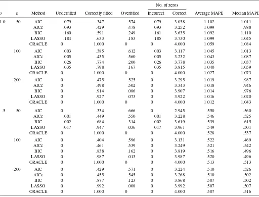
For each parameter setting, a total of 1,000 simulation itera-tions are carried out to evaluate the finite-sample performance of LAD-lasso. The simulation results are summarized in Ta-bles 1–3, which include the percentage of correctly (under/over) estimated numbers of regression models, together with the aver-age number of correctly (mistakenly) estimated 0’s, in the same manner as done by Tibshirani (1996) and Fan and Li (2001). Also included are the mean and median of themean absolute
prediction error(MAPE), evaluated based on another 1,000 in-dependent testing samples for each iteration.
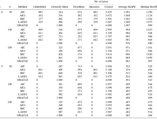
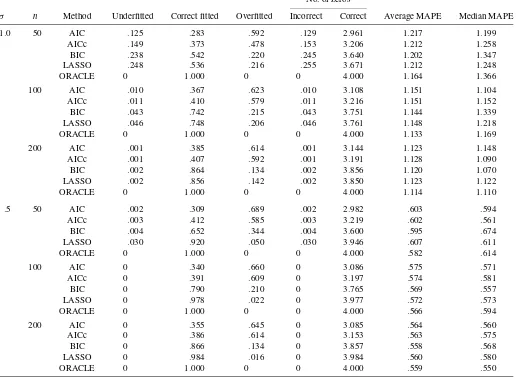
As can be seen from Tables 2–4, all of the methods (AIC, AICc, BIC, and LAD-lasso) demonstrate comparable predic-tion accuracy in terms of mean and median MAPE. However, the selection results differ significantly. In the case ofσ=1.0, both the AIC and AICc demonstrate appreciable overfitting ef-fects, whereas the BIC and LAD-lasso have very comparable performance, with both demonstrating a clear pattern of finding the true model consistently. Nevertheless, in the case ofσ=.5, LAD-lasso significantly outperforms the BIC with a margin that can be as large as 30% (e.g.,n=50; see Table 3) whereas the overfitting effect of the BIC is quite substantial.
Keep in mind that our simulation results should not be mis-takenly interpreted as evidence that the AIC (AICc) is an infe-rior choice compared with the BIC or LAD-lasso. As pointed out earlier, the AIC (AICc) is a well-known efficient but incon-sistent model selection criterion that is asymptotically optimal if the underlying model is of infinite dimension. On the other hand, the BIC and LAD-lasso are useful consistent model selec-tion methods if the underlying model is indeed of finite dimen-sion. Consequently, all of the methods are useful for practical data analysis. Our theory and numerical experience suggest that
Table 1. Simulation results for double-exponential error
No. of zeros
σ n Method Underfitted Correctly fitted Overfitted Incorrect Correct Average MAPE Median MAPE
1.0 50 AIC .079 .347 .574 .079 3.038 1.102 1.011 AICc .093 .429 .478 .093 3.252 1.099 .988 BIC .160 .591 .249 .161 3.635 1.092 1.110 LASSO .184 .633 .183 .185 3.730 1.099 1.045 ORACLE 0 1.000 0 0 4.000 1.059 1.084
100 AIC .003 .385 .612 .003 3.117 1.045 1.013 AICc .005 .435 .560 .005 3.232 1.043 1.087 BIC .026 .774 .200 .026 3.778 1.035 1.037 LASSO .035 .798 .167 .035 3.815 1.040 1.059 ORACLE 0 1.000 0 0 4.000 1.027 1.073
200 AIC 0 .475 .525 0 3.295 1.019 .987
AICc 0 .498 .502 0 3.343 1.018 .946
BIC 0 .914 .086 0 3.907 1.014 .976
LASSO 0 .927 .073 0 3.922 1.016 1.020 ORACLE 0 1.000 0 0 4.000 1.012 1.043
.5 50 AIC 0 .334 .666 0 2.945 .550 .560
AICc .001 .449 .550 .001 3.228 .546 .525 BIC .002 .684 .314 .002 3.619 .539 .615 LASSO .017 .947 .036 .017 3.961 .549 .501
ORACLE 0 1.000 0 0 4.000 .528 .537
100 AIC 0 .404 .596 0 3.131 .522 .469
AICc 0 .461 .539 0 3.249 .521 .542
BIC 0 .838 .162 0 3.819 .516 .496
LASSO 0 .987 .013 0 3.987 .520 .496
ORACLE 0 1.000 0 0 4.000 .513 .513
200 AIC 0 .429 .571 0 3.224 .510 .526
AICc 0 .455 .545 0 3.268 .510 .502
BIC 0 .877 .123 0 3.868 .507 .502
LASSO 0 .992 .008 0 3.992 .507 .507
ORACLE 0 1.000 0 0 4.000 .507 .516
Table 2. Simulation results fort5error
No. of zeros
σ n Method Underfitted Correctly fitted Overfitted Incorrect Correct Average MAPE Median MAPE
1.0 50 AIC .082 .244 .674 .082 2.825 1.052 1.290 AICc .102 .316 .582 .102 3.072 1.048 1.124 BIC .177 .492 .331 .179 3.501 1.042 1.164 LASSO .225 .566 .209 .228 3.687 1.048 1.073
ORACLE 0 1.000 0 0 4.000 1.007 .990
100 AIC .009 .316 .675 .009 2.995 .994 1.023 AICc .011 .364 .625 .011 3.105 .994 .948 BIC .027 .721 .252 .027 3.707 .985 .988 LASSO .042 .787 .171 .042 3.803 .991 .965
ORACLE 0 1.000 0 0 4.000 .976 .980
200 AIC 0 .323 .677 0 3.051 .971 1.161
AICc 0 .350 .650 0 3.104 .971 .986
BIC 0 .826 .174 0 3.814 .966 1.020
LASSO 0 .861 .139 0 3.856 .969 1.059
ORACLE 0 1.000 0 0 4.000 .963 .907
.5 50 AIC 0 .287 .713 0 2.904 .522 .525
AICc .001 .405 .594 .001 3.189 .519 .494 BIC .001 .660 .339 .001 3.596 .512 .544 LASSO .012 .963 .025 .012 3.975 .524 .489
ORACLE 0 1.000 0 0 4.000 .501 .522
100 AIC 0 .301 .699 0 2.957 .499 .546
AICc 0 .354 .646 0 3.090 .498 .475
BIC 0 .727 .273 0 3.700 .493 .493
LASSO 0 .982 .018 0 3.982 .495 .524
ORACLE 0 1.000 0 0 4.000 .489 .509
200 AIC 0 .325 .675 0 2.999 .487 .473
AICc 0 .348 .652 0 3.052 .486 .464
BIC 0 .800 .200 0 3.781 .483 .496
LASSO 0 .987 .013 0 3.987 .482 .514
ORACLE 0 1.000 0 0 4.000 .482 .494
LAD-lasso is a useful consistent model selection method with performance comparable to or even better than that of BIC, but with a much lower computational cost.
4. EARNINGS FORECAST STUDY
4.1 The Chinese Stock Market
Whereas the problem of earnings forecasting has been exten-sively studied in the literature on the North American and Eu-ropean markets, the same problem regarding one of the world’s fastest growing capital markets, the Chinese stock market, re-mains not well understood. China resumed its stock market in 1991 after a hiatus of 4 decades. Since it reopened, the Chinese stock market has grown rapidly, from a few stocks in 1991 to more than 1,300 stocks today, with a total of more than 450 bil-lion U.S. dollars in market capitalization. Many international institutional investors are moving into China looking for better returns, and earnings forecast research has become extremely important to their success.
In addition, over the past decade, China has enjoyed a high economic growth rate and rapid integration into the world mar-ket. Operating in such an environment, Chinese companies tend
to experience more turbulence and uncertainties in their opera-tions. As a result, they tend to generate more extreme earnings. For example, in our dataset, the kurtosis of the residuals dif-ferentiated from an OLS fit is as large as 90.95, much larger than the value 3 of a normal distribution. Hence the reliability of the usual OLS-based estimation and model selection meth-ods (e.g., AIC, BIC, lasso) is severely challenged, whereas the LAD-based methods (e.g., LAD, LAD-lasso) become more at-tractive.
4.2 The Dataset
The dataset used here is derived from CCER China Stock Database, which was partially developed by the China Cen-ter for Economic Research (CCER) at Peking University. It is considered one of the most authoritative and widely used stock market databases on the Chinese stock market. The dataset con-tains a total of 2,247 records, with each record corresponding to one yearly observation of one company. Among these, 1,092 come from year 2002 and serve as the training data, whereas the rest come from year 2003 and serve as the testing data.
The response variable is the return on equity (ROE), (i.e., earnings divided by total equity) of the following year
352 Journal of Business & Economic Statistics, July 2007
Table 3. Simulation results fort3error
No. of zeros
σ n Method Underfitted Correct fitted Overfitted Incorrect Correct Average MAPE Median MAPE
1.0 50 AIC .125 .283 .592 .129 2.961 1.217 1.199 AICc .149 .373 .478 .153 3.206 1.212 1.258 BIC .238 .542 .220 .245 3.640 1.202 1.347 LASSO .248 .536 .216 .255 3.671 1.212 1.248 ORACLE 0 1.000 0 0 4.000 1.164 1.366
100 AIC .010 .367 .623 .010 3.108 1.151 1.104 AICc .011 .410 .579 .011 3.216 1.151 1.152 BIC .043 .742 .215 .043 3.751 1.144 1.339 LASSO .046 .748 .206 .046 3.761 1.148 1.218 ORACLE 0 1.000 0 0 4.000 1.133 1.169 200 AIC .001 .385 .614 .001 3.144 1.123 1.148 AICc .001 .407 .592 .001 3.191 1.128 1.090 BIC .002 .864 .134 .002 3.856 1.120 1.070 LASSO .002 .856 .142 .002 3.850 1.123 1.122 ORACLE 0 1.000 0 0 4.000 1.114 1.110
.5 50 AIC .002 .309 .689 .002 2.982 .603 .594
AICc .003 .412 .585 .003 3.219 .602 .561 BIC .004 .652 .344 .004 3.600 .595 .674 LASSO .030 .920 .050 .030 3.946 .607 .611
ORACLE 0 1.000 0 0 4.000 .582 .614
100 AIC 0 .340 .660 0 3.086 .575 .571
AICc 0 .391 .609 0 3.197 .574 .581
BIC 0 .790 .210 0 3.765 .569 .557
LASSO 0 .978 .022 0 3.977 .572 .573
ORACLE 0 1.000 0 0 4.000 .566 .594
200 AIC 0 .355 .645 0 3.085 .564 .560
AICc 0 .386 .614 0 3.153 .563 .575
BIC 0 .866 .134 0 3.857 .558 .568
LASSO 0 .984 .016 0 3.984 .560 .580
ORACLE 0 1.000 0 0 4.000 .559 .550
(ROEt+1), and the explanatory variables include ROE of the
current year (ROEt), asset turnover ratio (ATO), profit mar-gin (PM), debt-to-asset ratio or leverage (LEV), sales growth rate (GROWTH), price-to-book ratio (PB), account receiv-ables/revenues (ARR), inventory/asset (INV), and the loga-rithm of total assets (ASSET). These are all measured at yeart.
Past studies on earnings forecasting show that these ex-planatory variables are among the most important accounting variables in predicting future earnings. Asset turnover ratio measures the efficiency of the company using its assets; profit margin measures the profitability of the company’s operation; debt-to-asset ratio describes how much of the company is
fi-Table 4. Estimation results of the earning forecast study
Variable AIC AICc BIC LAD-lasso LAD OLS
Int −.316809 −.316809 −.316809 −.363688 −2.103386 ROEt .207533 .207533 .207533 .067567 .190330 −.181815 ATO .058824 .058824 .058824 .006069 .058553 .165402
PM .140276 .140276 .140276 .134457 .209346
LEV −.020943 −.020943 −.020943 −.023592 −.245233 GROWTH .018806 .018806 .018806 .019068 .033153
PB .001544 .018385
ARR −.002520 .009217
INV .012297 .354148
ASSET .014523 .014523 .014523 .002186 .016694 .101458
MAPE .121379 .121379 .121379 .120662 .120382 .233541 STDE .021839 .021839 .021839 .022410 .021692 .021002
NOTE: “−” represents insignificant variable.
nanced by creditors rather than shareholders; and sales growth rate and price-to-book ratio measure the actual past growth and expected future growth of the company. The account receiv-able/revenues ratio and the inventory/asset ratio have not been used prominently in studies of North American or European companies, but we use them here because of the observation that Chinese managers have much more discretion over a com-pany’s receivable and inventory policies, as allowed by account-ing standards. Therefore, it is relatively easy for them to use these items to manage the reported earnings and influence earn-ings predictability. We include the logarithm of total assets for the same reason, because large companies have more resources under control, which can be used to manage earnings.
4.3 Analysis Results
Various methods are used to select the best model based on the training dataset of 2002. The prediction accuracies of these methods are measured by the MAPE based on the testing data for 2003. For the AIC and BIC, the best subset selection is car-ried out. For comparison purposes, the results of the full model based on the LAD and OLS estimators are also reported; these are summarized in Table 4.
As can be seen, the MAPE of the OLS is as large as .233541. It is substantially worse than all other LAD-based methods, fur-ther justifying the use of the LAD methods. Furfur-thermore, all of the LAD-based selection criteria (i.e., AIC, AICc, and BIC) agree that PB, ARR, and INV are not important, whereas LAD-lasso further identifies the intercept together with PM, LEV, and GROWTH as insignificant variables. Based on a substantially simplified model, the prediction accuracy of the LAD-lasso es-timator remains very satisfactory. Specifically, the MAPE of the LAD-lasso is .120662, only slightly larger than the MAPE of the full LAD model (.120382). According to the reported stan-dard error of the MAPE estimate (STDE), we can clearly see that such a difference cannot be statistically significant. Conse-quently, we conclude that among all of the LAD-based model selection methods, LAD-lasso resulted in the simplest model with a satisfactory prediction accuracy.
According to the model selected by LAD-lasso, a firm with high ATO tends to have higher future profitability (positive sign of ATO). Furthermore, currently more profitable compa-nies continue to earn higher earnings (positive coefficient on ROEt). Large companies tend to have higher earnings because they tend to have more stable operations, occupy monopolistic industries, and have more resources under control to manage earnings (positive sign of ASSET). Not coincidentally, these three variables are the few variables that capture a company’s core earnings ability the most: efficiency (ATO), profitability (ROEt), and company size (Assets) (Nissim and Penman 2001). It is natural to expect that more accounting variables would also have predictive power for future earnings in developed stock markets such as the North American and European markets. However, in a new emerging stock market with fast economic growth, such as the Chinese stock market, it is not surprising that only the few variables, which capture a company’s core earnings ability the most, would survive our model selection and produce accurate predictions.
5. CONCLUDING REMARKS
In this article we have proposed the LAD-lasso method, which combines the ideas of LAD and lasso for robust regres-sion shrinkage and selection. Similar ideas can be further ex-tended to Huber’s M-estimation using the following ψ-lasso objective function:
ψ-function contains the LAD function | · |as a special case,
ψ-lasso would be expected to be even more efficient than LAD-lasso if an optimal transitional point could be used. How-ever, for real data, how to select such an optimal transitional point automatically within a lasso framework is indeed a chal-lenging and interesting problem. Further study along this line is definitely needed.
ACKNOWLEDGMENTS
The authors are grateful to the editor, the associate editor, the referees, Rong Chen, and W. K. Li for their valuable comments and constructive suggestions, which led to substantial improve-ment of the manuscript. This research was supported in part by the Natural Science Foundation of China (grant 70532002).
APPENDIX A: PROOF OF LEMMA 1
We want to show that for any givenǫ >0, there exists a large constantCsuch that piecewise linear, the inequality (A.1) implies, with probabil-ity at least 1−ǫ, that the LAD-lasso estimator lies in the ball {β+n−1/2u:u ≤C}. For convenience, we define Dn(u)≡ other hand, according to Knight (1998), it holds that forx=0, |x−y| − |x|
= −y[I(x>0)−I(x<0)] +2
y
0 [
I(x≤s)−I(x≤0)]ds.
354 Journal of Business & Economic Statistics, July 2007
Applying the foregoing equation,Ln(u)can be expressed as
−n−1/2u′
By the central limit theorem, the first item on the right side of (A.3) converges in distribution tou′W, whereWis a p -di-mensional normal random vector with mean0and variance
ma-trix=cov(x1).
Next we show that the second item on the right side of (A.3) converges to a real function ofu in probability. Denote
the cumulative distribution function of ǫi by F and the item
n−1/2u′xi
On the other hand, due to the continuity off, there existη >0 and 0< κ <∞such that sup|x|<ηf(x) <f(0)+κ. Then it can
It follows from the law of large numbers that
n
where “→p” represents “convergence in probability.” There-fore, the second item on the right side of (A.3) converges to
f(0)u′uin probability.
By choosing a sufficiently largeC, for (A.3), the second item dominates the first item uniformly in u =C. Furthermore, the second item on the last line of (A.2) converges to 0 in prob-ability and hence is also dominated by the second item on the right side of (A.3). This completes the proof of Lemma 1.
APPENDIX B: PROOF OF LEMMA 2
Using a similar argument as that of Bloomfield and Steiger (1983, p. 4), it can be seen that the LAD-lasso criterionQ(β)
is piecewise linear and reaches the minimum at some breaking point. Taking the first derivative ofQ(β)at any differentiable pointβ˜ =(β˜1, . . . ,β˜p)′with respect toβj,j=p0+1, . . . ,p, we
By the central limit theorem, it is obvious that
V(0)=n−1/2
n
i=1
xisgn(ǫi)→dN(0,),
where “→d” represents “convergence in distribution.” Note that
n−1/2max {|u′xi|}n
i=1=op(1), and lemma A.2 of Koenker and
Zhao (1996) can be applied, which leads to
sup ≤M|
V()−V(0)+f(0)| =op(1),
where M is any fixed positive number. Then for any β˜ =
(β˜′a,β˜b′)′satisfying that√n(β˜a−βa)=Op(1)and| ˜βb−βb| ≤
where∗=√n(β˜−β). Hence
APPENDIX C: PROOF OF THE THEOREM
For any v=(v1, . . . ,vp0)′ ∈R we know that the first item at the right side of (A.1),
n
where W0 is a p0-dimensional normal random vector with
mean0and variance matrix0. Furthermore,
n
tion. Hence the required central limit theorem follows from lemma 2.2 and remark 1 of Davis et al. (1992). This completes the proof of the theorem.
[Received March 2005. Revised February 2006.]
REFERENCES
Akaike, H. (1973), “Information Theory and an Extension of the Maximum Likelihood Principle,” in2nd International Symposium on Information The-ory, eds. B. N. Petrov and F. Csaki, Budapest: Akademia Kiado, pp. 267–281. Bassett, G., and Koenker, R. (1978), “Asymptotic Theory of Least Absolute Error Regression,” Journal of the American Statistical Association, 73, 618–621.
Bloomfield, P., and Steiger, W. L. (1983),Least Absolute Deviation: Theory, Applications and Algorithms, Boston: Birkhauser.
Craven, P., and Wahba, G. (1979), “Smoothing Noise Data With Spline Func-tion: Estimating the Correct Degree of Smoothing by the Method of Gener-alized Cross Validation,”Numerische Mathematik, 31, 337–403.
Davis, R. A.. Knight, K., and Liu, J. (1992), “M-Estimation for Autoregres-sions With Infinite Variance,”Stochastic Process and Their Applications, 40, 145–180.
Fan, J., and Li, R. (2001), “Variable Selection via Nonconcave Penalized Like-lihood and Its Oracle Properties,”Journal of the American Statistical Asso-ciation, 96, 1348–1360.
Hurvich, C. M., and Tsai, C. L. (1989), “Regression and Time Series Model Selection in Small Samples,”Biometrika, 76, 297–307.
(1990), “Model Selection for Least Absolute Deviation Regression in Small Samples,”Statistics and Probability Letters, 9, 259–265.
Knight, K. (1998), “Limiting Distributions forL1Regression Estimators Under General Conditions,”The Annals of Statistics, 26, 755–770.
Knight, K., and Fu, W. (2000), “Asymptotics for Lasso-Type Estimators,”The Annals of Statistics, 28, 1356–1378.
Koenker, R., and Zhao, Q. (1996), “Conditional Quantile Estimation and Infer-ence for ARCH Models,”Econometric Theory, 12, 793–813.
Ling, S. (2005), “Self-Weighted Least Absolute Deviation Estimation for Infi-nite Variance Autoregressive Models,”Journal of the Royal Statistical Soci-ety, Ser. B, 67, 1–13.
McQuarrie, D. R., and Tsai, C. L. (1998),Regression and Time Series Model Selection, Singapore: World Scientific.
Nissim, D., and Penman, S. (2001), “Ratio Analysis and Equity Valuation: From Research to Practice,”Review of Accounting Studies, 6, 109–154. Peng, L., and Yao, Q. (2003), “Least Absolute Deviation Estimation for ARCH
and GARCH Models,”Biometrika, 90, 967–975.
Pollard, D. (1991), “Asymptotics for Least Absolute Deviation Regression Es-timators,”Econometric Theory, 7, 186–199.
Schwarz, G. (1978), “Estimating the Dimension of a Model,”The Annals of Statistics, 6, 461–464.
Shao, J. (1997), “An Asymptotic Theory for Linear Model Selection,”Statistica Sinica, 7, 221–264.
Shi, P., and Tsai, C. L. (2002), “Regression Model Selection: A Residual Likelihood Approach,”Journal of the Royal Statistical Society, Ser. B, 64, 237–252.
(2004), “A Joint Regression Variable and Autoregressive Order Selec-tion Criterion,”Journal of Time Series, 25, 923–941.
Tibshirani, R. J. (1996), “Regression Shrinkage and Selection via the LASSO,”
Journal of the Royal Statistical Society, Ser. B, 58, 267–288.
Tibshirani, R., Saunders, M., Rosset, S., Zhu, J., and Knight, K. (2005), “Spar-sity and Smoothness via the Fused Lasso,”Journal of the Royal Statistical Society, Ser. B, 67, 91–108.
Zou, H., Hastie, T., and Tibshirani, R. (2004), “On the ‘Degrees of Freedom’ of Lasso,” technical report, Standford University, Statistics Department.