Full Terms & Conditions of access and use can be found at
http://www.tandfonline.com/action/journalInformation?journalCode=ubes20
Download by: [Universitas Maritim Raja Ali Haji] Date: 12 January 2016, At: 23:48
Journal of Business & Economic Statistics
ISSN: 0735-0015 (Print) 1537-2707 (Online) Journal homepage: http://www.tandfonline.com/loi/ubes20
Panel and Pseudo-Panel Estimation of
Cross-Sectional and Time Series Elasticities of Food
Consumption
François Gardes, Greg J Duncan, Patrice Gaubert, Marc Gurgand &
Christophe Starzec
To cite this article: François Gardes, Greg J Duncan, Patrice Gaubert, Marc Gurgand & Christophe Starzec (2005) Panel and Pseudo-Panel Estimation of Cross-Sectional and Time Series Elasticities of Food Consumption, Journal of Business & Economic Statistics, 23:2, 242-253, DOI: 10.1198/073500104000000587
To link to this article: http://dx.doi.org/10.1198/073500104000000587
Published online: 01 Jan 2012.
Submit your article to this journal
Article views: 157
Panel and Pseudo-Panel Estimation of
Cross-Sectional and Time Series Elasticities
of Food Consumption: The Case of
U.S. and Polish Data
François G
ARDESUniversité de Paris I Panthéon-Sorbonne (Cermsem), Paris, 75005, France (gardes@univ-paris1.fr)
Greg J. D
UNCANNorthwestern University, Evanston, IL 60208 (greg-duncan@northwestern.edu)
Patrice G
AUBERTUniversité du Littoral (LEMMA), Boulogne sur Mer Cedex, 62321, France (gaubert@univ-paris1.fr)
Marc G
URGANDCNRS–Delta, Paris, 75014, France (gurgand@delta.ens.fr)
Christophe S
TARZECCNRS–TEAM, Paris, 75013, France (starzec@univ-paris1.fr)
This article addresses the problem of the bias of income and expenditure elasticities estimated on pseudo-panel data caused by measurement error and unobserved heterogeneity. We gauge these biases empirically by comparing cross-sectional, pseudo-panel, and true panel data from both Polish and U.S. expenditure surveys. Our results suggest that unobserved heterogeneity imparts a downward bias to cross-section estimates of income elasticities of at-home food expenditures and an upward bias to estimates of income elasticities of away-from-home food expenditures. “Within” and first-difference estimators suffer less bias, but only if the effects of measurement error are accounted for with instrumental variables. KEY WORDS: AIDS model; Individual and grouped data; Unobserved heterogeneity.
1. INTRODUCTION
A multitude of data types and econometric models can be used to estimate demand systems. Data types include aggregate time series, within-group time series, cross-sections, pseudo-panels using aggregated data, and cross-sections and pseudo-panels using individual data. Aggregate time series data frequently produce aggregation biases because of composition effects due to the change of the population or the heterogeneity of price and income effect between different social classes. These prob-lems have led the vast majority of empirical studies in labor economics to use individual data (Angrist and Krueger 1999).
In contrast,individualpanel data generally span short time periods and are subject to nonresponse attrition bias. Even pan-els on countries or industrial sectors can suffer from structural changes or composition effects that make it difficult to maintain the stationarity hypotheses for all variables.
Thus, grouping data to estimate on a pseudo-panel is an al-ternative, even when panel data exist, to estimate on longer pe-riods or to compare different countries. Pseudo-panel data are typically constructed from a time series of independent surveys that have been conducted under the same methodology on the same reference population but in different periods, sometimes consecutive and sometimes not.
In pseudo-panel analyses, individuals are grouped according to criteria that do not change from one survey to another, such
as their birth year or the education level of the reference per-son of a household. Estimation with pseudo-panel data dimin-ishes efficiency on the cross-sectional dimension, but we show herein that it also gives rise to a heteroscedasticity in the time dimension.
Static and dynamic demand models have been developed for these different types of data, with each model adopting a differ-ent approach to problems caused by unobserved heterogeneity across consumption units or time period of measurement, as well as the cross-equation restrictions imposed by consumption theory. Using different types of data helps reveal the nature of the biases that they impart to estimates of income and expendi-ture elasticities.
This article addresses the issue of bias to income and ex-penditure elasticities caused by errors of specification, mea-surement, and omitted variables or by heteroscedasticity in grouped and individual-based models. We gauge these biases by estimating static expenditure models using cross-sectional, pseudo-panel, and true panel data from both Polish and U.S. expenditure surveys. To our knowledge, this is the first com-parison between cross-sectional, pseudo-panel, and panel es-timations based on the same dataset. The use of one of our
© 2005 American Statistical Association Journal of Business & Economic Statistics April 2005, Vol. 23, No. 2 DOI 10.1198/073500104000000587 242
two datasets—the Panel Study of Income Dynamics (PSID)— is motivated by the numerous expenditure studies based on it (Altug and Miller 1990; Altonji and Siow 1987; Hall and Mishkin 1982; Naik and Moore 1996; Zeldes 1989). Our sec-ond dataset is from Poland in the late 1980s, which enables us to capitalize on large income and price variations during the transition period in Poland.
Section 2 presents a background discussion. Section 3 presents the econometric problems and describes the methods used in this study. Section 4 describes the data. Section 5 gives the results, and Section 6 discusses these results.
2. BACKGROUND
No matter how complete, survey data on household expen-ditures and demographic characteristics lack explicit measures of all of the possible factors that might bias the estimates of in-come and price elasticities. For example, the value of time dif-fers across households and is positively related to a household’s observed income. Because consumption activities (e.g., eating meals) often involve inputs of both goods (e.g., groceries) and time (e.g., time spent cooking and eating), households will face different (full) prices of consumption even if the prices of the goods-based inputs are identical. If—as is likely in the case of meals prepared at home—these prices are positively asso-ciated with income and themselves have a negative effect on consumption, then the omission of explicit measurement of full prices will impart a negative bias to the estimated income elas-ticities. The same argument can be applied to the case of virtual prices arising from, say, liquidity constraints that are most likely in low-income households (Cardoso and Gardes 1996). Taking into account the virtual prices appearing from nonmonetary re-sources such as time, or restricting the choice space due to con-straints applying only to subpopulations, or changing from one period to another, may help us better identify and understand cross-sectional and time series estimation differences.
Panel data on households provide opportunities to reduce these biases, because they contain information on changes in expenditures and income for the same households. Differencing successive panel waves nets out the biasing effects of unmea-sured persistent characteristics. But while reducing bias due to omitted variables, differencing income data is likely to magnify another source of bias: measurement error. Altonji and Siow (1987) demonstrated the likely importance of measurement er-ror in the context of first-difference consumption models by showing that estimates of income elasticities are several times higher when income change is instrumented than when it is not. Deaton (1986) presented the case for using “pseudo-panel” data to estimate demand systems. He assumed that the re-searcher has independent cross-sections with the required expenditure and demographic information and shows how cross-sections in successive years can be grouped into compa-rable demographic categories and then differenced to produce many of the advantages gained from differencing individual panel data. Grouping into cells tends to homogenize the in-dividual effects among inin-dividuals grouped in the same cell, so that the average specific effect is approximately invariant between two periods and is efficiently removed by within or first-difference transformations.
We evaluate implications of alternative approaches to esti-mating demand systems using two sets of household panel ex-penditure data. The two panels provide us with data needed to estimate static expenditure models in first-difference and “within” forms. However, these data can also be treated as though they came from independent cross-sections and from grouped rather than individual household-level observations. Thus we are able to compare estimates from a wide variety of data types. Habit persistence and other dynamic factors give rise to dynamic models (e.g., Naik and Moore 1996). We estimated dynamic versions of the static models using usual instrumen-tation methods (Arrelano 1989) and found that elasticity esti-mates were quite similar to those estimated for the static models presented in this article. However, these dynamic versions are questionable in terms of the specification and the econometric problems, so we prefer to consider only the static specification. True panel and pseudo-panel methods each offers advantages and disadvantages for handling the estimation problems inher-ent in expenditure models. A first set of concerns cinher-enters on measurement error. Survey reports of household income are measured with error; differencing reports of household income across waves undoubtedly increases the extent of error. Instru-mental variables can be used to address the biases caused by measurement error (Altonji and Siow 1987). Like instrumenta-tion, aggregation in pseudo-panel data helps reduce the biasing effects of measurement error, so we expect the income elastic-ity parameters estimated with pseudo-panel data to be similar to those estimated on instrumented income using true panel data. Because measurement error is not likely to be serious in the case of variables like location, age, social category, and family composition, we confine our instrumental variables adjustments to our income and total expenditure predictors. Measurement errors in our dependent expenditure variable are included in model residuals and, unless correlated with the levels of our in-dependent variables, should not bias the coefficient estimates.
Special errors in measurement can appear in pseudo-panel data when corresponding cells do not contain the same individ-uals in two different periods. Thus if the first observation for cell 1 during the first period is an individual A, then it will be paired with a similar individual B observed during the second period, so that measurement error arises between this observa-tion of B and the true values for A if he or she had been observed during the second period.
Deaton (1986) treated this problem as a measurement error; sample-based cohort averages are error-ridden measures of true cohort averages. He proposed a Fuller-type correction to en-sure convergence of pseudo-panel estimates. However, Verbeek and Nijman (1993) showed that Deaton’s estimator converges with the number of time periods. Moreover, Le Pellec and Roux (2002) showed that the measurement error correction variance matrix used in Deaton’s estimator is often not positive defi-nite in the data. The simpler pseudo-panel estimator used in this article has been shown to converge with the cell sizes (Verbeek and Nijman 1993; Moffit 1993), because measure-ment error becomes negligible when cells are large. Based on simulations, Verbeek and Nijman (1993) argued that cells must contain about 100 individuals, although the cell sizes may be smaller if the individuals grouped in each cell are sufficiently homogeneous.
Resolving the measurement error problem by using large samples within cells creates another problem: loss of efficiency of the estimators. This difficulty was shown by Cramer (1964) and Haitovsky (1973) with estimations based on grouped data and by Pakes (1983) with the problem induced by an omitted variable with a group structure, which is similar to the problem of measurement error.
The answer to the efficiency problem is to define group-ings that are optimal in the sense of keeping efficiency losses to a minimum but also keeping measurement error ignorably small (Baltagi 1995). Grouping methods were developed by Cramer (1964), Haitovsky (1973), Theil and Uribe (1967), and Verbeek and Nijman (1993) that involve carefully choosing co-horts to obtain the largest reduction of heterogeneity within each cohort but at the same time maximizing the heterogene-ity between them. Following these empirical principles, using pseudo-panels leads to consistent and efficient estimators with-out the problems associated with true panels. Our work groups individuals into cells that are both homogeneous and large.
Second, the aggregation inherent in pseudo-panel data pro-duces a systematic heteroscedasticity. This can be corrected exactly by decomposing the data into between and within di-mensions and computing the exact heteroscedasticity on both dimensions. But because the heteroscedastic factor depends on time, correcting it by generalized least squares (GLS) makes individual-specific effects vary with time, thus canceling the spectral decomposition in between and within dimensions. This can result in serious estimation errors (Gurgand, Gardes, and Bolduc 1997). The approximate correction of heteroscedastic-ity that we use involves weighting each observation by a het-eroscedasticity factor that is a function of, but not exactly equal to, cell size. Thus the least squares coefficients computed on the grouped data may differ slightly from those estimated on individual data. As described in the next section, this approxi-mate and easily implemented correction uses GLS on the within and between dimensions with a common variance–covariance matrix, computed as the between transformation of the het-eroscedastic structure due to aggregation.
Third, unmeasured heterogeneity is likely to be present in both panel and pseudo-panel data. In the case of panel data, the individual-specific effect for householdhisα(h), which is assumed to be constant through time. In the case of pseudo-panel data, the individual-specific effects for a household (h)
belonging to the cell(H)at periodtcan be written as the sum of two orthogonal effects, α(h,t)=µ(H)+υ(h,t). Note that the second component depends on time, because the individuals composing the cellHchange through time.
The specific effectµcorresponding to the cellH[µ(H)] rep-resents the influence of unknown explanatory variablesW(H), constant through time, for the reference group H, which is defined here by the cell selection criteria. Here υ(h,t) are individual-specific effects containing effects of unknown ex-planatory variables Z(h,t). In the pseudo-panel data, the ag-gregated specific effect ζ (H)for the cell H is defined as the aggregation of individual-specific effects,
ζ (H,t)=γ (h,t)×α(h,t)=µ(H)+γ (h,t)×υ(h,t),
wheretindicates the observation period andγis the weight for the aggregation ofhwithin cells. Note that the aggregate, but not individual-specific, effects depend on time.
The within and first-difference operators estimated with panel data cancel the individual-specific effectsα(h). The com-ponentµ(H)is also canceled on pseudo-panel data by the same operators, whereas the individual effectυ(h,t)may be largely eliminated by the aggregation. Thus it can be supposed that the endogeneity of the specific effect is greater on individual than on aggregated data, because aggregation cancels a part of this effect.
Therefore, with panel data, the within and the first-difference operators suppress all of the endogeneity biases. With pseudo-panel data, the same operator suppresses the endogeneity due toµ, but not that due toγ (h,t)
×υ(h,t). For each individual, this part of the residual may be smaller relative toµ, because cell homogeneity is increased. Conversely, the aggregation into cells is likely to cancel this same componentυ across individ-uals, so it is not easy to predict the effect of the aggregation on the endogeneity bias.
Our search for robust results is facilitated by the fact that the two panel datasets that we use cover extremely different societies and historical periods. One dataset is from the United States for 1984–1987, a period of steady and substantial macro-economic growth. The other is from Poland for 1987–1990, a turbulent period that spans the beginning of Poland’s tran-sition from a command to a free-market economy.
3. SPECIFICATION AND ECONOMETRICS OF THE CONSUMPTION MODEL
Data constraints force us to estimate a demand system on only two commodity groups over a period of 4 years: food con-sumed at home and food concon-sumed away from home. Away-from-home food expenditures are rare in the Polish data, so our estimates are not very reliable, but we keep them to compare them with PSID estimates. We use the almost-ideal demand system (AIDS) developed by Deaton and Muellbauer (1980), with a quadratic form for the natural logarithm of total income or expenditures to take nonlinearities into account.
Note that the true quadratic system proposed by Banks, Blundell, and Lewbel (1997) implies much more sophisticated econometrics if the nonlinear effect of prices is taken into ac-count. It may be difficult to precisely estimate the price effect because of the short estimation period in the PSID data. On the other hand, our Polish dataset contains relative prices for food that change both across 16 quarters and between 4 so-cioeconomic classes. Thus we estimated the linearized version of Quadratic Almost Ideal System (QAIDS) (with the Stone index) on the Polish panel, using the convergence algorithm proposed by Banks et al. (1997) to estimate the integrability parametere(p)in the coefficient of the quadratic log income [see (1)]. We obtained very similar income elasticities for food consumed at home and food consumed away from home to those obtained by the linear AIDS model. The AIDS estimates for both countries are presented in Tables 1 and 2. The ad-ditivity constraint is automatically imposed by ordinary least squares (OLS).
The possible correlation between the residuals of food con-sumed at home and food concon-sumed away from home would suggest the use of seemingly unrelated regression (SUR). We tested this possible correlation on Polish data and found no significant difference between OLS and SUR estimations.
Table 1. Income Elasticities for Food at Home and Away From Home: PSID (1984–1987)
Between Cross-sections Within First differences
Panel Food at home
Not instrumented .167 (.008) .140 (.017) −.019 (.019) −.029 (.034) Instrumented
Whole population .010 (.027) −.030 (.054) .363 (.082) .473 (.158) Robust estimation .187 (.025) .134 (.050) .383 (.077) .447 (.150) Food away
Not instrumented .963 (.019) .872 (.039) −.025 (.043) .062 (.063) Instrumented
Whole population 1.046 (.043) .966 (.094) .375 (.166) .431 (.260) Robust estimation 1.050 (.044) .960 (.095) .387 (.166) .447 (.258) Surveys 1984–1985–1986–1987
n 9,720
Control variables Age, equivalence scale, and its square
Pseudo-panel (not instrumented) Food at home
(a) .311 (.045) .265 (.056) .240 (.095) .382 (.114)
(b) .306 (.033) .460 (.062)
Food away
(a) 1.387 (.068) 1.265 (.083) .800 (.150) .847 (.172) (b) 1.384 (.060) 1.125 (.127)
Surveys 1984–1985–1986–1987
n 90
Control variables Log of age and its square, equivalence scale and its square
NOTE: The values in parentheses are standard errors adjusted for the instrumentation of total expenditures by the usual method.
Because relative prices do not vary much within waves of the same survey compared with the variations between different years (at least for the U.S. in the mid-1980s), even if we con-sider quarterly variations of prices, we account for price effects and other macroeconomic shocks with survey year dummies for the U.S. data. For the Polish data, we gave each individual a price index differentiated by social category and the quarter of the year in which he or she was surveyed.
Our model takes the form
wiht=ai+biln(Yht/pt)+ci/e(p)[ln(Yht/pt)]2+Zhtdi+uiht,
(1) wherewihtis the expenditure budget share on goodiby house-holdhat time t,Yht is its income in the case of the U.S. data
or logarithmic total expenditure in the case of the Polish data,
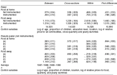
Table 2. Total Expenditure Elasticities for Food at Home and Away From Home: Polish Surveys (1987–1990)
Between Cross-sections Within First differences
Panel Food at home
Not instrumented .579 (.004) .536 (.009) .466 (.005) .451 (.010) Instrumented .494 (.010) .567 (.023) .755 (.013) .788 (.028) Food away
Not instrumented 1.119 (.073) 1.239 (.164) 2.618 (.556) 1.460 (.185) Instrumented 1.216 (.143) 1.326 (.329) 4.195 (1.080) 1.315 (.393)
n 14,520 14,520 14,520 10,890
Control variables Log of age, proportion of children, education level, location, log of relative price for all commodities, cross-quarterly and yearly dummies
Pseudo-panel (not instrumented) Food at home
(a) .583 (.011) .572 (.017) .549 (.020) .864 (.033)
(b) .591 (.010) .584 (.022)
(c) .591 (.011) .581 (.018) .526 (.020) .568 (.033) (d) .589 (.013) .581 (.018) .965 (.023) .915 (.032) Food away
(a) .820 (.203) .890 (.258) −.218 (.318) .696 (.331)
(b) .609 (.208) −.529 (.331)
(c) .608 (.213) .240 (.270) −.072 (.322) .333 (.508) (d) 1.149 (.212) .367 (.268) .624 (.199) .965 (.315) Surveys 1987–1988–1989–1990
n 224
Control variables Log of age, proportion of children, location, log of relative prices for food, quarterly, and yearly dummies
NOTE: The values in parentheses are standard errors adjusted for the instrumentation of total expenditures by the usual method.
pt is the Stone price index, Zht is a matrix of socioeconomic
characteristics and survey year or quarter dummies, and
e(p)=
i
pbi
it
is a factor estimated by the convergence procedure proposed by Banks et al. (1997) that ensures the integrability of the demand system. When using total expenditure data from the Polish panel, the allocation of income between consumption and saving can be ignored, and total expenditures can be con-sidered a proxy for permanent income. Our U.S. data do not provide information on total expenditure, so that income elas-ticities are computed on the basis of total household disposable income. Using income instead of total expenditures would be better served by a model in which income is decomposed into permanent and transitory components.
Our cross-sectional estimates of (1) are based on data on indi-vidual households from each available single-year cross-section (1984–1987 in the case of the PSID and 1987–1990 in the case of the Polish expenditure survey).
First-difference and within operators are procedures com-monly used to eliminate biases caused by persistent omit-ted variables. We use our panel data to obtain first-difference and within estimates of our model. Following Altonji and Siow (1987), we estimate our models both with and with-out instrumenting for change in log income or expenditures. Instrumenting income from the PSID is necessary because of likely measurement errors observed in such income data. We also instrument the total expenditure from the Polish surveys, because measurement errors for both total expenditures and food expenditures are likely correlated.
In the QAIDS specification, the classical errors-in-variables cannot hold for the squared term if it holds for the log of in-come. As far as we know, this problem has not been yet solved conveniently, so we simply used the square of the instrumented income, checking that a separate instrumentation of the squared term does not significantly change the results.
For cross-sections and first-differences, we found two types of correlations, between individuals in cross-sections and be-tween periods in first differences. We consider this problem by estimating separately for each period using a robust OLS method. For the within estimation, all autoregressive processes on the residuals (resulting, e.g., from partial adjustment in ex-ogenous variables) are taken into account, as was suggested by Hsiao (1986, pp. 95–96), by estimating the system of equations written for the successive periods.
The grouping of data for pseudo-panels is based on six age cohorts and two or three education levels. The grouping of households (h,t)in the cells(H,t)gives rise to the exact
ag-h ∈ H (a natural hypothesis, according to the grouping of households into a same H cell). A heteroscedasticity factor
δHt=h∈Hγht2 arises for the residualεi, which is due to the
change of cell sizes (as γ ∼= |H1| if the two grouping crite-ria homogenize the household’s total expenditures). Thus the
grouping of data builds up a heteroscedasticity that may change over time because of the variation in cell sizes. In Appendix A we show that this heteroscedasticity cannot be corrected by usual methods.
We present exact correction procedures in Appendix A and show that under a symmetry condition, heteroscedasticity also can be approximately corrected by simple GLS based on the average heteroscedasticity factor over time for each cell,
T
In our datasets, the size variation through time for each cell is unimportant, so the heteroscedasticity factor due to the grouping is quite invariant. In this article, heteroscedasticity is corrected by the exact procedure for within and between estimations, and also by simple GLS based on the average heteroscedasticity factor for all estimations.
For PSID data, the population is randomly divided into four subsamples, each of which is used to aggregate data for the dif-ferent years. This prevents the same household from being in-cluded in the same cell in more than one period (in which case the aggregation would correspond just to grouped panel data).
For the Polish data, all households (after filtering for some outliers defined on sectional estimations) in the cross-sectional component of each survey are used for the pseudo-panelization; panel households belonging to the surveys are excluded. The sample size for each year is around 27,000 house-holds, much larger than for the PSID data.
The PSID cells sizes vary from 9 to 183 households, with a mean of 65.5, and from 8 to 60, with a mean of 25.1, for the Polish data. Fourteen of the 72 cells constituting the whole pseudo-panel in the PSID contain fewer than 30 households, representing only 4% of the whole population. Because the correction for the heteroscedasticity on the pseudo-panel data involves weighting each cell by weights close to its size, esti-mation without these small cells gives the same results as those for the whole. For each cell, the size variation over time is much less important, so that the heteroscedasticity factor due to the grouping is quite invariant through time.
It is clear that the residuals for two adjacent equations esti-mated in first differences,(uih,t−uih,t−1)and(uih,t−1−uih,t−2), are systematically correlated. Because all specifications are es-timated by Zellner’s seemingly unrelated regressions, our pro-cedures take into account the correlation between the residuals of the two food components.
Price effects are taken into account by period dummies for the PSID and by price elasticities for Poland. The head of household’s age and family size and structure are also taken into account in the estimations. Adding other control variables, such as head of household’s sex, education level, wealth, and employment status, in the PSID had very little effect on the es-timates. We selected only age and family structure variables for the PSID, to make the estimations comparable to the results based on the Polish data.
Correction for grouped heteroscedasticity may still leave some heteroscedasticity for the estimations at the individual level. We test for this by regressing the squared residuals on a quadratic form of explanatory variables, thus correcting it when
necessary by weighting all observations by the inverse absolute residual. The coefficient on the squared income is generally sig-nificant, but QAIDS estimates are very close to AIDS estimates.
4. DATA
4.1 The Panel Study of Income Dynamics
Each year since 1968, the PSID has followed and interviewed a national sample that began with about 5,000 U.S. families (Hill 1992). The original sample consisted of two subsamples: an equal-probability sample of about 3,000 households drawn from the Survey Research Center’s dwelling-based sampling frame, and a sample of low-income families that had been in-terviewed in 1966 as part of the U.S. Census Bureau’s Survey of Economic Opportunity and who consented to participate in the PSID.
When weighted, the combined sample is designed to be continuously representative of the nonimmigrant population as a whole. To avoid problems that might be associated with the low-income subsample, our estimations based on individual-household data are limited to the (unweighted) equal-probability portion of the PSID sample. To maximize within-cell sample sizes, our pseudo-panel estimates are based on the combined total weighted PSID sample. We note in-stances when pseudo-panel estimates differed from those based on the equal-probability portion of the PSID sample.
Because income instrumentation requires lagged measures from two previous years, our 1982–1987 subset of PSID data provides us with data spanning five cross-sections (1983–1987). We used only 4 years in estimating the consumption equation to be comparable with the Polish data. In all cases the data were restricted to households in which the head did not change over the 6-year period and to households with major imputations on neither food expenditure nor income variables. In terms of the PSID’s “accuracy” imputation flags, we excluded cases with codes of 2 for income measures and of 1 or 2 for food at home and food away from home measures.
To construct cohorts for the pseudo-panels, we defined a se-ries of variables based on the age and education level of the household head. Specifically, we defined six cohorts of age of household head (under 30 years, 30–39, 40–49, 50–59, 60–69, and over 69) and three levels of education of household head (did not complete high school, completed high school but had no additional academic training, and completed at least some university-level schooling).
The PSID provides information on two categories of expen-diture (food consumed at home and food consumed away from home) and has been used in many expenditure studies (e.g., Hall and Mishkin 1982; Altonji and Siow 1987; Zeldes 1989; Altug and Miller 1990; Naik and Moore 1996). These expenditures are reported by the households as an estimation of their yearly consumption, so reporting zero consumption can be considered a true no consumption. That is why no correction of selection bias is needed.
All of these studies were based on the cross-sectional analy-ses and thus may be biased because of the endogeneity prob-lems discussed earlier. To adjust expenditures and income for family size, we use the Oxford equivalence scale: 1.0 for the
first adult, .8 for the other adults, .5 for the children over age 5 years, and .4 for children under age 6 years. Our expenditure equations also include a number of household structure vari-ables to provide additional adjustments for possible expenditure differences across different family types.
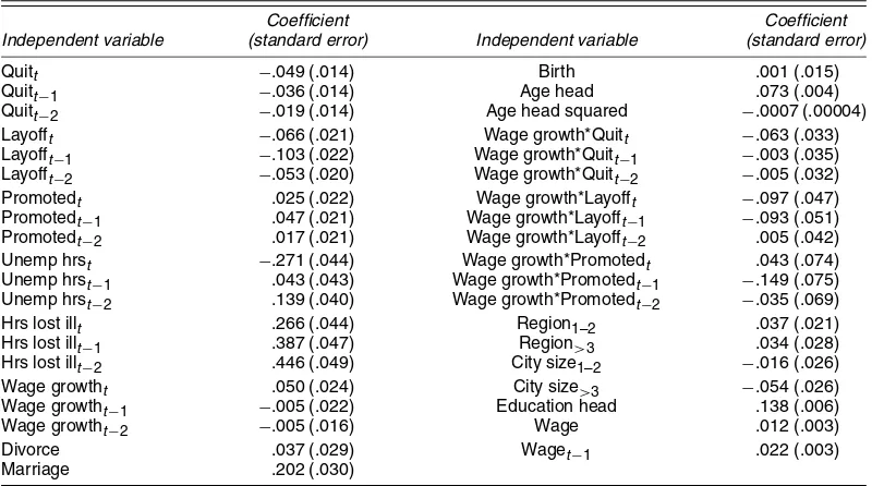
Disposable income is computed as total annual household cash income plus food stamps minus household payments of al-imony and child support to dependents living outside the house-hold and minus income taxes paid (the househouse-hold’s expenditure on food bought with food stamps is also included in our mea-sure of at-home food expenditure). As instruments for levels of disposable income, we follow Altonji and Siow (1987) in in-cluding three lags of quits, layoffs, promotions, and wage-rate changes for the household head (and constructing our wage rate measure from a question sequence about rate of hourly pay or salary that is independent of the question sequence that pro-vides the data on disposable household income), as well as changes in family composition other than the head, marriage and divorce/widowhood for the head, and city size and region dummies. For first-difference models, the change in dispos-able income is instrumented using the first-difference of instru-mented income in level.
Means and standard deviations of the PSID variables are pre-sented in Table A.1; coefficients and standard errors from the first stage of the instrumental variables procedure are presented in Table A.2.
4.2 The Polish Expenditure Panel
Household budget surveys have been conducted in Poland for many years. In the period analyzed (1987–1990), the an-nual total sample size was about 30 thousand households, ap-proximately .3% of all the households in Poland. The data were collected using a rotation method on a quarterly basis. The master sample comprises households and persons living in randomly selected dwellings. To generate it, a two-stage and (in the second stage) two-phase sampling procedure was used. The full description of the master sample–generating procedure was given by Lednicki (1982).
Master samples for each year contain data from four differ-ent subsamples. Two subsamples began their interviews in 1986 and ended the 4-year survey period in 1989. They were replaced by new subsamples in 1990. Another two subsamples of the same size were started in 1987 and followed through 1990.
Over this 4-year period, it is possible to identify house-holds participating in the surveys during all 4 years. These households form a 4-year panel. There is no formal identifi-cation possibility (by number) of this repetitive participation, but special procedures allowed us to specify the 4-year par-ticipants with a very high probability. The checked and tested number of households is about 3,707 (3,630 after some filter-ing). The available information is as detailed as for the cross-sectional surveys: all typical sociodemographic characteristics of households and individuals, as well as details on incomes and expenditures, are measured. The expenditures are reported for 3 consecutive months each year, so we considered again that zero expenditure is a true no-consumption case. Thus no cor-rection is needed for selection bias, like for the PSID.
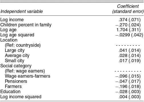
Comparisons between reported household income and re-cord-based information showed a number of large discrepan-cies. For employees of state-owned and cooperative enterprises (who constituted more than 90% of wage earners until 1991), wage and salary incomes were checked at the source (em-ployers). Kordos and Kubiczek (1991) estimated that employ-ees’ income declarations for 1991 were 21% lower on average than employers’ declarations. Generally, the proportion of un-reported income decreases with the level of education and in-creases with age. In cases where declared income was lower than that reported by enterprises, household income was in-creased to the level of the reported income. Because income measures are used only to form instrumental variables in our expenditure equations, the measurement error is likely to cause only minor problems.
Table A.3 presents descriptive information on the Polish data, and Table A.4 presents coefficients from the instrumental vari-ables equation. The period 1987–1990 covered by the Polish data is unusual even in Polish economic history. It represents the shift from the centrally planned, rationed economy (1987) to a relatively unconstrained fully liberal market economy (1990). Gross domestic product (GDP) grew by 4.1% between 1987 and 1988, but fell by .2% between 1988 and 1989 and by 11.6% between 1989 and 1990. Price increases across these pairs of years were 60.2%, 251.1%, and 585.7%. Thus the transition years 1988 and 1989 produced a period of a very high infla-tion and a mixture of free-market, shadow, and administrated economy.
This means that the consumers’ market reactions could have been highly influenced by these unusual situations. This is most likely the case for the year 1989, when uncertainty, inflation, market disequilibrium, and political instability reached their highest levels. Moreover, in 1989 and 1990 individuals were facing large real income fluctuations, as well as dramatic changes in relative prices. This unstable situation produced atypical consumption behaviors of households facing a sub-sistence constraint. This may be the case of very-low-income households facing a dramatic decrease in their purchasing power (>30%).
5. RESULTS
Estimates from our various models are presented in Tables 1 (PSID) and 2 (Polish surveys). Respective columns show in-come for PSID and total expenditure for the Polish data, along with elasticity estimates for between, cross-sectional (com-puted as the means of cross-sectional estimates obtained on each cross-sectional survey), within, and first-difference mod-els. Results are also presented separately for models in which income or total expenditure is and is not instrumented using the models detailed in Tables A.2 and A.4. We expect the between estimates to be similar to the average of cross-sectional esti-mates. Compared with the within estimates, the first-difference estimates may be biased by greater measurement error, but the specific effects may be better taken into account whenever they change within the period.
For the PSID, we eliminated some observations to obtain robust estimations using the DFBETAS explained by Belsley,
Kuh, and Welsch (1980) to select outliers. We eliminated obser-vation whenDFBETAS>2/√n, wherenis the number of ob-servations. Rejected observations represent 4% of the sample.
For the Polish data, estimation of a QAIDS model by it-eration on the integrability parameter (see Banks et al. 1997) gives very similar results, except for food away (between and within estimators). The QAIDS estimations are very close to the results presented in Table 2. Filtering data for outliers (like for PSID) did not significantly change the results.
For pseudo-panel data, heteroscedasticity has been corrected by the approximate method (GLS with a heteroscedasticity fac-torδH, that is constant through time) [Tables 1 and 2, (a)], and
the exact method [Tables 1 and 2, (b)] presented in Appendix A. Also given in Appendix A are the estimates obtained without correction [Table 2, (c)] and with a false correction (GLS with a heteroscedasticity factor δHt) [Table 2, (d)] for the Polish
pseudo panel data. The between and cross-sectional estimates are similar for the different correction methods, especially for food at home, but the within and first-differences estimates ob-tained under the false correction, which is currently used in pseudo-panel estimations, gives very different estimates than those computed for the approximate correction, the exact cor-rection, or no correction. Thus correction for heteroscedasticity seems to be an important methodological point in the estimation on pseudo-panel data. The false correction gives very different estimates, especially for time series estimations. However, in our case the exact correction gives rise to estimated parameters close to those obtained by the approximate correction, so we principally discuss these estimates that can be easily compared under the spectral decomposition into the between and within dimensions.
Looking first at the PSID results for at-home food expen-ditures, it is quite apparent that elasticity estimates are very sensitive to adjustments for measurement error and unmea-sured heterogeneity. Cross-sectional estimates of at-home in-come elasticities are low (between .15 and .30) but statistically significant without or with instrumentation (when performing robust estimations). The between estimates effectively average the cross-sections and also produce low estimates of elasticities. Pseudo-panel data produces similar elasticities for between and cross-sectional estimates. Despite some variations among the different estimations, the relative income elasticity of food at home is around .20 based on this collection of methods.
Within and first-difference estimates of PSID-based in-come elasticities are around 0 without instrumentation and around .40 with instrumentation. A Hausman test strongly re-jects (pvalue< .01) the equality of within and between esti-mates (Table 3). The test compares within and GLS estiesti-mates; equivalently, it can be built from the within and between es-timates (see Baltagi 1995, p. 69). The test is computed by the usual quadratic form, with a chi-squared distribution, with
Vdefined as the variance of the difference between the esti-mators tested,(βb−βw)′(V−1)(βb−βw), whereβ=(βly)or
β=(βly, βly2)for the quadratic estimation on the Polish panel
andV=Vb+Vwcorresponds to all the explanatory variables.
Note that a test withVas a matrix 2×2 computed only for the two income variables would be biased.
Because the within and first difference models adjust for per-sistent heterogeneity and the instrumentation adjusts for mea-surement error, .40 is our preferred approximate estimate of the
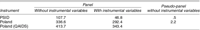
Table 3. Hausman Test for Income Parameters (food at home)
Panel Pseudo-panel
without instrumental variables Instrument Without instrumental variables With instrumental variables
PSID 107.7 46.8 .5
Poland 336.6 292.4 2.2
Poland (QAIDS) 413.7 343.4
income elasticity of at-home food expenditures in the United States. This is roughly double the sizes of the corresponding be-tween and cross-sectional parameter estimates, suggesting that failure to adjust for heterogeneity imparts a considerably down-ward bias to cross-sectional estimates. PSID-based pseudo-panel data also produce significantly (according to a Hausman test) higher elasticity estimates for first differences compared with between and cross-sections models, although there is little consistency across the full set of pseudo-panel estimates.
Expenditure elasticities for at-home food estimated with the Polish data are much higher in value than the income elastic-ity estimates based on PSID data. (Note that the Polish elas-ticities are computed on total expenditures, so they must be multiplied by the income elasticity of total expenditures, which is around .7, to be compared to the PSID income elasticities.) Higher elasticities are to be expected for a country in which food constitutes a share of total expenditures that is three times higher than that in the United States (Tables A.1 and A.3). Their consistency probably stems from the smaller degree of measurement error in the Polish expenditure than in the PSID income data. Before the households were grouped into cells, 10 households were suppressed. The criterion for suppression was the prediction of food consumption in cross-sectional esti-mates. On the panel data, robust estimations produced by sup-pressing some outliers gave similar results to those obtained for the whole panel. Time series Polish pseudo-panel estimates were a little smaller than estimates based on the microdata. On the whole, the estimations on Polish data also produced higher within and first-difference elasticities than between and cross-sectional elasticities.
PSID-based income elasticities for away-from-home food expenditures are quite different from and even more sensitive to specification than the at-home food expenditure elasticity es-timates. Between and cross-sectional estimates are around 1.0 in both individual and pseudo-panel data. In contrast with the case of at-home expenditures, adjustments for heterogeneity through use of within and first-difference estimates produce much lower estimates. We speculate on why this might be the case in Section 6.
Polish food-away-from-home expenditures are reported in the survey relatively rarely and are very low even when com-pared with those for other countries with comparable income levels. Moreover, about 70% of these expenditures in the ob-served periods is spent on highly subsidized business can-teens and cafeterias. Thus the estimations should be compared with the food-away-from-home expenditure estimation in other countries with caution.
Price data in Poland enabled us to compute price elasticities. Quarterly price indices for four social categories were com-puted from the monthly GUS (Polish Main Statistical Office)
publication Biuletyn Statystyczny and imputed at the individ-ual level to the dataset. The variability of the prices both over time and over social categories provides good estimates of the direct compensated elasticity for food at home (around −1). In contrast with the income elasticities, the cross-sectional es-timates of direct price elasticities are close to those obtained from time series. As prices change between quarters and house-holds of different types, the only explanation of an endogeneity bias would be a correlation between household types and price levels. Such a correlation is less probable than the correlation between relative income and the specific component of food consumption (which produces the endogeneity bias on income elasticities). However, if systematically high (or low) price lev-els are correlated with household type (e.g., as in segmented markets), and if these types of households are characterized by a systematically positive or negative specific consumption, then the endogeneity bias can appear. This is not the case for Poland in 1987–1990.
6. DISCUSSION
We have attempted to assess the bias on income and expendi-ture elasticity estimates caused by inattention to measurement error and unobserved heterogeneity. In the case of U.S. at-home food expenditure elasticity, our preferred estimate is around .40. Failure to adjust for unmeasured heterogeneity and, in some cases, measurement error appears to impart a substantial down-ward bias to this estimate. These adjustments operate in the same direction for estimates of the at-home expenditure elas-ticity found in the Polish data.
In the case of U.S. away-from-home food expenditures, our preferred elasticity estimate is less certain but similar in mag-nitude to the .40 elasticity for at-home expenditures. (Note that it is considerably higher in pseudo-panel estimate.) Surprising here is the magnitude and sign (upward) of the apparent bias inherent in both individual and pseudo-panel estimates that do not adjust for unobserved heterogeneity.
Why should unmeasured heterogeneity induce an upward bias in away-from-home expenditures in the U.S. and Polish data? Earlier, we speculated that a likely downward bias for the at-home food elasticity estimates may be caused by fail-ure to account for the fact that the value of time differs across households and is positively related to the household’s ob-served income. The time input to producing at-home meals leads households to face different (full) prices of consump-tion even if the prices of the goods-based inputs are identi-cal. If these prices are positively associated with income and themselves have a negative effect on consumption, then their omission will impart a negative bias to the estimated income elasticities. Note that the bias seems somewhat less pronounced
on pseudo-panel data. The correlation between income and spe-cific effect may be decreased by aggregation, as we suggested in Section 2.
In the case of expenditures for meals consumed in restau-rants, there are large variations in the mixture of food and service components. Time spent consuming full-service restau-rant meals is typically longer than time spent consuming fast-food restaurant meals, but in this case higher-income households may well attach a more positive value to such time than low-income households. Failing to control for this source of heterogeneity will probably impart a positive bias to esti-mates of income elasticities. (Note that the endogeneity bias is much more pronounced for food away from home than for food at home.)
The use of time can be measured with the shadow price of time. This shadow price increases with household income, so that the complete price for food, computed as the sum of the monetary and shadow prices, increases also along the income distribution. Therefore, the difference between cross-sectional and time series income elasticities can be related to the change of this complete price. The argument is formalized in Appen-dix B.
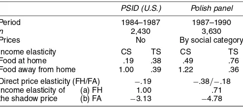
Calibrating the price effect as half of the income effect (as suggested by Frisch) and using (B.2) in Appendix B pro-duces an estimate of the income elasticity of the food shadow price (Table 4). It is remarkable that these elasticities are simi-lar in the two countries, positive and around 1 for food at home and negative and much larger for food away. Thus the time con-straint imparts much stronger relative changes in expenditures in restaurants than at home, which is normal because the budget shares of food away are much smaller in both countries (espe-cially in Poland, where the ratio of the price elasticities is the largest). A substitution between food at home and food away from home when the ratio of their complete prices changes im-parts a similar change in the expenditures, but greater changes in the food away from home budget share.
Elasticity estimates from the Polish data also proved some-what sensitive to adjustments for heterogeneity. This is not surprising given the very different price regimes in the Polish economy during this period, with one (presumably low) set of prices faced by the many farm families who have the option of growing their own food; official, subsidized prices set by the Polish government; and higher black market prices for the same or similar products. In fact, until 1988 the official prices of sta-ples, such as bread, were set so low that very few farm families grew food for their own consumption, when queuing was not a problem.
Table 4. Income Elasticity of Food Shadow Prices
PSID (U.S.) Polish panel
Period 1984–1987 1987–1990
n 2,430 3,630
Prices No By social category Income elasticity CS TS CS TS Food at home .19 .38 .49 .76 Food away from home 1.00 .39 1.22 .36 Direct price elasticity (FH/FA) −.19 −.38/−.18 Income elasticity of (a) FH 1.00 .71 the shadow price (b) FA −3.13 −4.78
Our estimates are based on a static consumption model and risk of bias due to the omission of dynamic factors, such as habit persistence. We investigated this by estimating a dynamic ver-sion of our model that included lagged consumption. To obtain cross-sectional estimates of our dynamic model, we treated our data as though they came from three independent 2-year panels (1984–1985 through 1986–1987 for the PSID and 1987–1988 through 1989–1990 for the Polish expenditure survey). We es-timated this dynamic model as a system using SURE and both with and without instrumentation for log total income or expen-diture and found that the coefficient on the lagged dependent variables were significant in these dynamic models, but their inclusion changed the values of the short-run income elasticity very little.
An important result of this work is that pseudo-panel esti-mates are often close to estiesti-mates based on genuine panel data. Large and similar apparent endogeneity biases were found in both countries. Cross-sectional estimations produce elasticities that are systematically higher for food at home and lower for food away from home. Moreover, it seems that the aggregation lowers the endogeneity bias for food consumption. Future re-search should aim to verify these results on a complete set of expenditure data. Once corrected for the biases, income elastic-ities for food at home and food away from home become very close to each other in the U.S. data, a result that seems rea-sonable to us and highlights possible errors that can arise from estimations using cross-sectional data.
ACKNOWLEDGMENTS
The authors gratefully acknowledge helpful suggestions from participants at seminars at the University of Michigan, Northwestern University, Université de Paris I, Université de Genève, Erudite, CREST, Journées de Microéconomie Ap-pliquée (1998), Congress of the European Economic Associ-ation, and International Conference on Panel Data, as well as research support from INRA, INRETS, and CREDOC. The Polish data were made available by Professor Górecki, Uni-versity of Warsaw, Department of Economics. The authors also thank CREST, INSEE, and MATISSE for support.
APPENDIX A: HETEROSCEDASTICITY IN THE PSEUDO–PANEL MODEL
Write the pseudo-panel model presented in the text in a ma-trix form as
y=Xβ+Zα+ε,
whereyis anNTcolumn vector withNthe number of cohorts andT the number of periods,Xis a matrix of explanatory vari-ables,βis a vector of parameters,Zis an (NT×N) matrix that contains cell dummies,αis a vector of cohort effects, andεis a heteroscedastic residual. CallDa diagonal (NT×NT) ma-trix such thatD=diag(δHt), whereδHtis defined as in the text
and varies with cell size and the within-cell structure of relative expenditure. The model variance matrix is thus
=σα2TB+σε2D,
Table A.1. Means and Standard Deviations of Variable Used in the PSID Analyses
1983 Level
1984 1985 1986 1987
Level Dif. Level Dif. Level Dif. Level Dif.
Budget share for .147 .144 −.003 .129 −.015 .137 .008 .134 −.003 food at home (.103) (.098) (.084) (.095) (.086) (.100) (.082) (.096) (.081) Percent with at-home
share=0 0 0 53.2 0 74.0 0 41.5 0 51.3
Budget share for .033 .034 .001 .031 −.003 .033 .002 .033 .001 food away from home (.040) (.038) (.034) (.038) (.033) (.041) (.032) (.034) (.033) Percent with away-from-home
share=0 9.5 8.9 5.7 9.6 5.5 10.3 5.5 8.9 5.7 ln household income 9.9254 9.9985 .0731 10.1714 .1729 10.1238 −.0475 10.1671 .0432
(.648) (.657) (.280) (.716) (.320) (.686) (.308) (.694) (.299) ln age head 3.7044 3.7306 .0262 3.7573 .0267 3.7801 .0228 3.8044 .0242
(.377) (.368) (.013) (.359) (.013) (.351) (.012) (.343) (.012) ln family size .6741 .6837 .0096 .6896 .0060 .6894 −.0002 .6912 .0018 (Oxford scale) (.404) (.401) (.162) (.405) (.168) (.409) (.159) (.410) (.171)
NOTE: The values in parentheses are standard errors.
Table A.2. Regression Coefficient and Standard Errors for Instrumental Variables Equation for Income Level for the PSID (dependent variable: disposable family income in logs in 1987, 1986, 1985)
Coefficient Coefficient
Independent variable (standard error) Independent variable (standard error)
Quitt −.049 (.014) Birth .001 (.015)
Quitt−1 −.036 (.014) Age head .073 (.004) Quitt−2 −.019 (.014) Age head squared −.0007 (.00004) Layofft −.066 (.021) Wage growth*Quitt −.063 (.033)
Layofft−1 −.103 (.022) Wage growth*Quitt−1 −.003 (.035) Layofft−2 −.053 (.020) Wage growth*Quitt−2 −.005 (.032) Promotedt .025 (.022) Wage growth*Layofft −.097 (.047) Promotedt−1 .047 (.021) Wage growth*Layofft−1 −.093 (.051) Promotedt−2 .017 (.021) Wage growth*Layofft−2 .005 (.042) Unemp hrst −.271 (.044) Wage growth*Promotedt .043 (.074)
Unemp hrst−1 .043 (.043) Wage growth*Promotedt−1 −.149 (.075) Unemp hrst−2 .139 (.040) Wage growth*Promotedt−2 −.035 (.069) Hrs lost illt .266 (.044) Region1–2 .037 (.021) Hrs lost illt−1 .387 (.047) Region>3 .034 (.028) Hrs lost illt−2 .446 (.049) City size1–2 −.016 (.026) Wage growtht .050 (.024) City size>3 −.054 (.026) Wage growtht−1 −.005 (.022) Education head .138 (.006) Wage growtht−2 −.005 (.016) Wage .012 (.003) Divorce .037 (.029) Waget−1 .022 (.003) Marriage .202 (.030)
NOTE: The values in parentheses are standard errors.
Table A.3. Means and Standard Deviations of Variables Used in the Polish Panel Analyses
1987 1988 1989 1990
Level Dif. Level Dif. Level Dif. Level Dif.
Budget share for .508 .484 −.024 .486 .003 .554 .068 food at home (.14) (.15) (.14) (.18) (.17) (.15) (.17) Percent with at-home
share>0 100 100 100 100 100 100 100
Budget share for .006 .006 −.001 .005 −.001 .005 .0002 food away from home (.02) (.03) (.02) (.02) (.02) (.03) (.03) Percent with away-from-home
share=0 28.4 29.7 26.9 20.5
ln household expenditure 10.65 11.17 .50 12.25 −.18 14.14 −.03 (.45) (.49) (.38) (.79) (.62) (.50) (.58) ln head’s age 3.789 3.809 .020 3.824 .014 3.842 .019 (.33) (.32) (.16) (.32) (.15) (.32) (.15) ln family size 1.140 1.121 −.019 1.095 −.026 1.081 −.014 (.59) (.60) (.24) (.61) (.21) (.61) (.22)
NOTE: The values in parentheses are standard errors.
Table A.4. Regression Coefficient and Standard Errors for Instrumental Variables Equation for Total Expenditure Level and Change for
the Polish Expenditure Panel
Coefficient
Independent variable (standard error)
Log income .374 (.071)
Children percent in family −.270 (.024)
Log age 1.704 (.311)
Log age squared −.0299 (.042) Location Wage earners-farmers −.096 (.015) Pensioners −.047 (.017) Farmers −.196 (.018) Education −.028 (.003) Log income squared .004 (.003)
NOTE: The values in parentheses are standard errors.
whereB is the between transformation matrix. The matrixD
in this expression is the source of cell and time-varying het-eroscedasticity.
The GLS estimator ofβis
ˆ
βGLS=(X′−1X)−1X′−1y.
In panel analysis, this can be expressed as a weighted sum of between and within estimators, which is calledspectral decom-position. This holds if−1can be projected into the within and between dimensions, that is, if matrices1and2exist such
that
−1=W1W+B2B.
Gurgand et al. (1997) showed that this can be the case only if matrixBis symmetric, which implies that the weights inD
are time-invariant. The intuition of this result is that if, in the process of scaling the variances, individual effects α receive differing weights for various observations of a given cohort, the within transformation no longer resolves individual heterogene-ity, so that it does not strictly reflect the time series variance of the model. DecomposingβˆGLS into the cross-sectional and time series dimensions based on the within and between esti-mates thus is no longer possible. In contrast, as long as cell size is constant over time, this argument does not hold, and the de-composition obtains.
A corollary is that the efficient within estimator cannot be based simply on the original model weighted by heteroscedas-ticity varying factors, because this would create time-varying cohort effects. Gurgand et al. (1997) showed that the within estimator that is both efficient and consistent when
αandXare correlated is
ˆ
βW=(X′WWX)−1X′WWy,
where = D−1 − D−1Z(Z′D−1Z)−1Z′D−1. Alternatively, when the number of cohorts is small, the least squares dummy variable estimator can be used, with weights directly propor-tional to δHt. The between estimator is straightforward
be-cause the time dimension is absent and is easily obtained by weighted least squares, with weights (σµ2+σε2wc/T)−.5 with
wc=1/TtδHt.
APPENDIX B: MEASURING THE SHADOW PRICES
Suppose that monetary price,pm, and a shadow price,π,
cor-responding to nonmonetary resources and to constraints faced by the households are combined into a complete price. Ex-pressed in logarithm form, we havepc=pm+π.
Two estimations of the same equation,
xiht=g(Zht)=Zht·βi+uiht, (B.1)
for good i (i=1, . . . ,n) and individual h (h=1, . . . ,H) in period t (t=1, . . . ,T) are made on cross-sectional and time series dimensions over the same dataset. The residual is de-composed between αih, the specific effect that contains all
permanent components of the residual for individual h and goodi, and the residual effectεiht:uiht=αih+εiht. The
cross-sectional estimates can be biased by a correlation between some among the explanatory variables Zht and this specific effect
(see Mundlak 1978). Such a correlation is due to latent per-manent variables (e.g., an event during infancy, characteris-tics of parents, or permanent wealth) which are related both to the specific permanent effect and to the between transfor-mation of the explanatory variables Zht. Note δi, the
correla-tion coefficient between the time average of the vector of the explanatory variables,Zht=(Zhtk)k=1,...,K1, transformed by the
between matrix BZht= {(1/T)tZhtk}k=1,...,K1, and the
spe-cific effectαih=BZht·δi+ηih. This coefficient adds to the
pa-rameterβicorresponding to the influence ofZin the between
estimation, Bxiht=BZht·(βi+δi)+ηih+Bεiht, so that the
between estimates are biased. Thus the difference between the cross-sectional and time series estimates is equal toδi.
Suppose that the shadow price depends on some among vari-ablesZ, for instance,Zhtk. The marginal propensity to consume with respect toZhtk when considering the effect of the shadow pricesπjhton consumption can be written as
dxiht/dZhtk =dgi/dZhtk +
propensity of endogeneous variables can be used to identify the shadow price variation overZkht,dπjht/dZhtk, because it can
be computed by resolving a system ofn linear equations after having estimated the price marginal propensitiesdgi/dπj=γij.
In our estimations we consider only thedirect effectthrough the price of goodi:γii·dπi/dZhtk, so that
dπi/dZhtk =
βi(c.s.)−βi(t.s.)
/γii. (B.2)
[Received September 2002. Revised August 2004.]
REFERENCES
Altonji, J., and Siow, A. (1987), “Testing the Response of Consumption to In-come Changes With (Noisy) Panel Data,”Quarterly Journal of Economics, 102, 293–328.
Altug, S., and Miller, R. (1990), “Household Choices in Equilibrium,” Econo-metrica, 58, 543–570.
Angrist, J. D., and Krueger, A. B. (1999), “Empirical Strategies in Labor Eco-nomics,” inHandbook of Labor Economics, Vol. 3A, eds. A. Ashenfelter and D. Card, Amsterdam: North-Holland, Chap. 23, pp. 1277–1366.
Arellano, M. (1989), “A Note on the Anderson–Hsiao Estimator for Panel Data,”Economic Letters, 31, 337–341.
Baltagi, B. H. (1988), “An Alternative Heteroscedastic Error Component Model Problem,”Econometric Theory, 4, 349–350.
(1995),Econometric Analysis of Panel Data, New York: Wiley. Banks, J., Blundell, R., and Lewbel, A. (1997), “Quadratic Engel Curves and
Consumer Demand,”The Review of Economics and Statistics, 79, 527–539. Belsey, D. A., Kuh, E., and Welsch, R. E. (1980),Regression Diagnostics:
Iden-tifying Influential Data and Sources of Collinearity, New York: Wiley. Blanciforti, L., and Green, R. (1983), “An Almost-Ideal Demand System
Incor-porating Habit Effect,”The Review of Economics and Statistics, 65, 511–515. Cardoso, N., and Gardes, F. (1996), “Estimation de Lois de Consommation sur un Pseudo-Panel d’Enquêtes de l’INSEE (1979, 1984, 1989),”Economie et Prévision, 5, 111–125.
Cramer, J. S. (1964), “Efficient Grouping, Regression, and Correlation in Engel Curve Analysis,”Journal of American Statistical Association, 59, 233–250. Deaton, A. (1986), “Panel Data From a Time Series of Cross-Sections,”Journal
of Econometrics, 30, 109–126.
Deaton, A., and Muellbauer, J. (1980),Economics and Consumer Behavior, Cambridge: Cambridge University Press.
Gardes, F., Langlois, S., and Richaudeau, D. (1996), “Cross-Section versus Time-Series Income Elasticities,”Economics Letters, 51, 169–175. Gorecki, B., and Peczkowski, M. (1992), “Polish Household Panel,”
unpub-lished manuscript, Warsaw University, Dept. of Economics.
Gurgand, M., Gardes, F., and Bolduc, D. (1997), “Heteroscedasticity in Pseudo-Panel,” unpublished working paper, Lamia, Université de Paris I.
Haitovsky, Y. (1973), Regression Estimation From Grouped Observations, New York: Hafner.
Hall, R., and Mishkin, F. (1982), “The Sensitivity of Consumption to Transi-tory Income: Estimates From Panel Data on Households,”Econometrica, 50, 261–281.
Hill, M. S. (1992),The Panel Study of Income Dynamics, a User’s Guide, Newburry Park, CA: Sage.
Hsiao, C. (1986),Analysis of Panel Data, Cambridge, U.K.: Cambridge Uni-versity Press.
Kordos, J. (1985), “Towards an Integrated System of Household Surveys in Poland,”Bulletin of International Statistical Institute, 51, 1.3-1–1.3.18. Kordos, J., and Kubiczek, A. (1991), “Methodological Problems in the
House-hold Budget Surveys in Poland,” Warsaw: GUS.
Lednicki, B. (1982), “Dobor Proby i Metoda Estimacji w Rotacyjnym Bada-niu Gospodarstw Domowych (Sample Design and Method of Estimation in Rotation Survey of Households),” GUS, Warsaw.
Le Pellec, L., and Roux, S. (2002), “Avantages et Limites des Méthodes de Pseudo-Panel: Une Analyse sur les Salaires des Ingénieurs Diplômés,” un-published working paper, CREST, 19th Journées de Micro-Économie Ap-pliquée, Rennes.
Mazodier, P., and Trognon, A. (1978), “Heteroscedasticity and Stratification in Error Components Models,”Annales de l’Insee, 30–31, 451–482.
Moffit, R. (1993), “Identification and Estimation in Dynamic Models With a Time Series of Repeated Cross-Sections,”Journal of Econometrics, 59, 99–123.
Mundlak, Y. (1978), “On the Pooling of Time Series and Cross-Section Data,”
Econometrica, 46, 483–509.
Naik, N. Y., and Moore, M. J. (1996), “Habit Formation and Intertemporal Sub-stitution in Individual Food Consumption,”The Review of Economics and Statistics, 78, 321–328.
Pakes, A. (1983), “On Group Effects and Errors in Variables in Aggregation,”
The Review of Economics and Statistics, 65, 168–173.
Theil, H., and Uribe, P. (1967), “The Information Approach to the Aggrega-tion of Input–Output Tables,”The Review of Economics and Statistics, 49, 451–462.
Verbeek, M., and Nijman, T. (1993), ”Minimum MSE Estimation of a Regres-sion Model With Fixed Effects From a Series of Cross-Sections,”Journal of Econometrics, 59, 125–136.
White, H. (1980), “A Heteroscedasticity Consistent Covariance Matrix Estima-tor and a Direct Test for Heteroscedasticity,”Econometrica, 48, 817–838. Zeldes, S. P. (1989), “Consumption and Liquidity Constraints: An Empirical
Investigation,”Journal of Political Economy, 97, 305–345.