Beta distributions in a simplex and impartial anonymous
cultures
* Eivind Stensholt
Norwegian School of Economics and Business Administration, Helleveien 30, 5035 Bergen-Sandviken, Norway
Received 30 June 1997; received in revised form 6 January 1998; accepted 11 February 1998
Abstract
Variations of IAC are introduced and simulated. A uniformly distributed point P5(X , X , . . . ,1 2
Xn11) in a simplex S is generated by a map (´1,´2, . . . ,´n)→P from the unit cube to S (surjective
with bijective restriction to interiors) with the´i’s rectangular and i.i.d on [0,1]. The fraction xyz of the electorate with preference x.y.z is a sum of X ’s. The variations allow differenti
correlations (e.g.r(xyz, xzy)±r(xyz, zyx) while they all are 20.2 under IAC. Simulation of two
such variations give smaller Condorcet paradox propability than IAC. This is explained heuristically with a graphic ‘‘pictogram’’ representation of the profile. 1999 Elsevier Science B.V. All rights reserved.
Keywords: Beta distributions; preference structures; Condorcet’s paradox; impartial anonymous cultures
JEL classification: D71
1. Introduction
Let a random point P5(X , X , . . . , X1 2 n11) be uniformly distributed in a simplex S. The sums of barycentric coordinates have beta-distributions, which are known as distributions for order statistics. In a recent paper, Tovey (1997) relates the order statistics directly to S and uses them to generate P. Section 2 generates P by a transformation Eq. (4) which also allows an elementary proof of the density formulas. The ‘‘cultures’’ IC and IAC, which are compared in Section 3, are common assumptions about the stochastic distribution of profiles. They are often used in
simulation work with the purpose of comparing the properties of various election rules which define the result in terms of the profile. Consider 3 alternatives a, b, c (parties, candidates, propositions). A profile for these alternatives is a vector Eq. (9) in the standard 5-dimensional simplex S, where xyz is the fraction of the electorate with preference order ‘‘x before y before z’’. This vector is multinomially distributed under the IC-assumption, and for a large electorate the distribution is concentrated around the simplex center. It is shown that if a, b, c are three among a larger number of alternatives, there is a similar concentration under IAC. For an election rule symmetric under all permutations of alternatives, all final rankings will then be equally probable, and any final ranking may be obtained for a profile arbitrarily close to the center.
Another common feature of IC and IAC is that the Condorcet paradox occurs much more often than it is seen in real life with large electorates. Section 4 suggests ways to use the easy generation of beta-distributions to define variations of the IAC which give a much smaller frequency of the paradox. In these cultures the x.y.z voters agree more
with the x.z.y voters than with the z.y.x voters etc. Two such variations are
studied with computer simulation. They have a much smaller paradox probability than the standard IAC. The ‘‘pictograms’’ of the profiles, introduced in Stensholt (1996), visualize the reason for this reduction.
2. Some probabilities associated with a simplex
Let S be an n-dimensional simplex with corners C , C , . . . , C1 2 n11. Let a stochastic point
P5(X ,X , . . . ,X1 2 n11)[S (1)
be distributed with uniform density in S. In Eq. (4) below is shown a way to generate Eq. (1) by means of a standard generator for a rectangularly distributed variable. The Xi
are the barycentric coordinates, so that C15(1, 0, . . . , 0)[S, etc. By definition,
Xi$0 for all i and X11X21 ? ? ? 1Xn1151. (2)
Since the barycentric coordinates are invariant under affine transformations, we may assume S is the standard simplex. Thus the X are stochastic variables identicallyi
distributed on the unit interval [0,1]. Also all the pairs (X , X ) with i±j are identically
i j
distributed, and similarly for triples, etc. Thus, by Eq. (2)
1 1
]] ]
E(X )i 5n11and Cov(X ,X )i j 5 2nVar(X ).i (3)
Let´1,´2, . . . ,´n be independent stochastic variables uniformly distributed on [0,1]. Then in Eq. (1) we obtain a uniformly distributed P[S by defining
1 / n 1 / n 1 / (n21 ) 1 / n 1 / (n21 )
(X ,X , . . . ,X1 2 n11)5(12´1 ,´1 ?(12´2 ),´1 ?´2
1 / (n22 ) 1 / n 1 / (n21 )
To establish this claim, observe that the event X1#x may be written equivalently
n
´ $1 (12x) . Hence the event x#X1#x1Dx has probability proportional to
n n n21
(12x) 2(12x2Dx) ¯n?Dx?(12x)
The claim follows by induction on n, the P[S with X15x forming an (n2 1)-dimensional simplex. The density function for each barycentric coordinate becomes
d d n n21
]dxProb(Xi#x)5]dx(12(12x) )5n?(12x) . (5)
From Eqs. (3) and (5) we obtain
n 21
]]]]] ]]]]]
Var(X )5 , Cov(X ,X )5 if i±j. (6)
i 2 i j 2
(n11) ?(n12) (n11) ?(n12)
Let Y be the sum of any t barycentric coordinates X , 1t i #t#n.
THEOREM The density function of Y ist
d n21 n2t t21
]dxProb(Yt#x)5n?
S D
t21 ?(12x) ?xFig. 1.
Comment: Eq. (4) defines a bijection between the interiors of the cube and the simplex
which maps equal volumes to equal volumes. The theorem states that Y has a standardt
form beta distribution with integer parameters (n112t, t). If the ´1, ´2, . . . , ´n are ordered by size: ´s( 1 )#´s( 2 )#. . .#´s(n), then t-th order statistic has the same distribution as Y . See Johnson et al. (1995, Ch. 25, 26). Tovey (1997) shows directlyi
that the vector of differences of the order statistics, in the above notation
(´s( 1 )2´s( 0 ),´s( 2 )2´s( 1 ), . . . ,´s(n11 )2´s(n))[S (´s( 0 )50,´s(n11 )51),
n2t t2n
is uniformly distributed. This gives an alternative way to generate P. Instead of the root extractions in Eq. (4) one then needs a sorting routine to finds.
Proof of Theorem: For t51, this is just Eq. (5). Without loss of generality, let
1 / n 1 / (n21 ) 1 / (n112t )
Yt5X11X21 . . . 1Xt512´1 ?´2 ? . . .?´t . (7) The proof now proceeds by induction on t, using the formula 12Yt115(12Y )t ?
1 / (n2t )
´t11 . Then, since ´t11 is rectangularly distributed on [0,1] and is also stochastically independent of Y , we gett
In election theory, particularly in simulation work as in Gehrlein (1997), Nurmi (1992) and Van Newenhizen (1992), various probabilities are introduced by assuming a ‘‘culture’’, i.e. a certain stochastic behaviour of the electorate. For each voter there is one ranking of a number of candidates, say N. The result is a ‘‘profile’’, i.e. a point Eq. (1) in the n-dimensional simplex S with n115N! corners. Then X is the fraction of thei
electorate which selects ranking no. i in some fixed ordering of the N! possible rankings.
Two frequently considered types of cultures are the following:
The impartial cultures (IC): Each voter independently picks a ranking at random, with probability 1 /(N!) for each. The profile Eq. (1) has a discrete (essentially multinomial) distribution which depends on the number of electors.
The impartial anonymous cultures (IAC): Each possible profile has the same probability. (The individual action of the voters is disregarded; they become ‘‘anonymous’’). Here we consider only the continuous case, i.e. the limit case when the number of voters tend to infinity. We thus assume the profile Eq. (1) to be uniformly and continuously distributed in S.
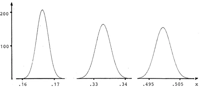
Fig. 2. The densities for the variables abc, abc1acb, abc1acb1cab.
a.b.c, a.c.b, c.a.b, c.b.a, b.c.a, b.a.c
corresponds one sixth of the n115N! rankings of all candidates. Let xyz be the fraction
of the electorate who choose a ranking with x.y.z. For our triple we get a profile (vote
vector)
(abc, acb, cab, cba, bca, bac) (9)
Under the continuous IAC, the components of Eq. (9) become stochastic variables which are disjoint sums of t5(n11) / 6 variables X in Eq. (1). With e.g. Ni 58 candidates, the densities for e.g. abc, abc1acb, abc1acb1cab are given by the
theorem with n58!21 and t58! / 6, 8! / 3, 8! / 2 respectively:
7892 33599 6719 11148 26879
0.13844214?10 ?(12x) ?x , 0.26288619?10 ?(12x) ?
13439 12140 20159 20159
x , 0.13553854?10 ?(12x) ?x .
The integral of the last expression from 0.49 to 0.51 is approx. 0.9999409; this is the probability that the outcome of a given pairwise contest (like a vs. c) is in the 0.49–0.51 range. See Fig. 2.
We are now ready to compare the assumptions of IAC and IC: Already for 8 candidates the IAC-profiles cluster around 1 / 6?(1,1,1,1,1,1)[S like the IC-profiles with
a large number of voters. The IAC-variance of abc1acb1cab, i.e. of Y with nt 115N!
and t5(n11) / 2, is calculated from Eqs. (6) and (7) as 1 /(4?(N!11)), which equals the IC-variance with 11N! voters, when (11N!)(abc1acb1cab) is binomial (0.5, 11N!).
As in Eq. (3), all IC-correlations between different components are also 20.2.
4. IAC and the Condorcet paradox. What is impartiality?
b beats a. For a simple geometric description of the paradox, rewrite the vector Eq. (9) expression Eq. (10) is unique; whether the paradox occurs depends only on the unit vector (v , v , v , v , v , v ). Provided this vector is uniformly distributed on the unit1 2 3 4 5 6
sphere, the paradox probability is
1 23
]?arc cos]¯0.08774; (11)
2p 27
see section 4.2 of Stensholt (1996). A sign change in the unit vector changes the cyclic order in the paradox. All cases where the joint density distribution of Eq. (9) is invariant under all rotations about the simplex center satisfy the uniformity condition.
Comment: ‘‘Guilbaud’s number’’ Eq. (11) (Guilbaud, 1968, p. 54) was found as the
limit probability for the Condorcet paradox with an increasing number of voters in an IC-culture. The IC profile is multinomially distributed, and making use of a multinormal approximation one may obtain Guilbaud’s result as a consequence of the mentioned result in Nurmi, 1992.
Under the IC with the number of voters increasing to infinity, the limit probability for the paradox is Eq. (11). For the continuous IAC with 3 candidates the paradox probability is 1 / 16. For a fixed alternative tripleha,b,cjin sets of 4 and 5 candidates, the computer simulation reported in Table 1 below shows that the paradox probability increases. The simulation values are, respectively, 0.0807595 and 0.0862578. The joint density distribution of Eq. (9) is very symmetrical, being invariant under the 6!5720 permutations of the simplex corners. It seems reasonable to conjecture that the limit distribution of the unit vector is uniform, and that Eq. (11) thus is the limit value for an increasing number of candidates under a continuous IAC.
Tables 1 and 2 are organized as Table 3 in Stensholt (1996). Thus, from Table 1 (3
2
candidates out of 5), line 4 tells us that there were 7 923 619 profiles with´,0.04 , out
2
of which 1 328 597 had ´$0.03 . Among these again, 151 203 profiles caused the Condorcet paradox to occur. Here´is the relative size of the triangle in the pictogram; see Stensholt (1996).
Comment on pictograms: The pictogram of the profile Eq. (9) consists of a circle and
Table 1
IAC-simulation results for:
3 candidates out of 4 3 candidates out of 5
01 1 183 930 1 183 930 757 2 536 861 2 536 861 8 844
Such profiles fit relatively well with a pie-sharing model where the alternatives a, b, c are represented as points in the disk, and the three mid-normals are chords which subdivide the disk into six areas approximately proportional to abc, acb, cab, cba, bca,
Table 2
Topic related IAC-simulation results for:
3 candidates, 24 topics 3 candidates, 24 topics
pattern A pattern B
in total 220 749 in total 168 412
own ‘‘ideal point’’ and the alternative points a,b,c. The alternative triangle abc is unique only up to a homothetic transformation centered on the chords’ intersection point.
Another interpretation of the pie-sharing when ´50 is to say that the chords’ intersection P represents ‘‘the present day policy’’, and that the alternatives a, b, c point out different directions from P. Consider unit vectors PA, PB, PC in these directions and let a point Q in the disk belong to the area representing abc if the inner products satisfy
PA?PQ$PB?PQ$PC?PQ etc. (Fig. 3B). This interpretation is natural if we assume
that each elector basically has preferences on the directions in which the policy may be changed.
Opinion poll data therefore seem to fit reasonably well with both assumptions, i.e. with ranking by distance and with ranking by direction. In Fig. 3 the (constructed) profile is
(abc, acb, cab, cba, bca, bac)5(0.29 0.14 0.08 0.28 0.20 0.11),´ 50.0000061 . . .
Based on the profile alone, one cannot argue that one interpretation is better than the other.
A pictogram discussion of the paradox: However, the probability Eq. (11) is very
unrealistic. The pictogram discussion of the paradox and the real data analysis in Stensholt (1996) show that the paradox for a randomly chosen alternative triple will be a very rare event in a large electorate, and will occur only in cases where all pairwise comparisons are close to 50–50. The main point is to observe that the paradox can only occur if the center of the pictogram circle is inside the small triangle of area´, as e.g. in Fig. 4A.
Stensholt
/
Mathematical
Social
Sciences
37
(1999
)
45
–
57
53
Table 3 Correlations
Pattern A: abc5SX withi Pattern B: abc5SX withi
i51, 2, 3, 4, 5, 6, 7, 8, 9, 10, 12 i51, 3, 4, 5, 6, 6, 7, 7, 8, 9, 10, 12
abc acb cab cba bca bac abc acb cab cba bca bac
abc 1 1 / 3 21 / 3 21 21 / 3 1 / 3 1 1 / 5 22 / 5 23 / 5 22 / 5 1 / 5
acb 1 / 3 1 1 / 3 21 / 3 21 21 / 3 1 / 5 1 1 / 5 22 / 5 23 / 5 22 / 5
cab 21 / 3 1 / 3 1 1 / 3 21 / 3 21 22 / 5 1 / 5 1 1 / 5 22 / 5 23 / 5 cba 21 21 / 3 1 / 3 1 1 / 3 21 / 3 23 / 5 22 / 5 1 / 5 1 1 / 5 22 / 5 bca 21 / 3 21 21 / 3 1 / 3 1 1 / 3 22 / 5 23 / 5 22 / 5 1 / 5 1 1 / 5
Fig. 3.
probability, but the more the profiles are concentrated, the smaller ´will be. Clearly a small´ favours a small paradox probability. Guilbaud’s number expresses the balance between the two opposite tendencies for the class of profile distributions, i.e. cultures, with a uniformly distributed unit vector in Eq. (10).
However, the clustering of Eq. (9) near the simplex center is not the whole explanation. It is very unrealistic to assume a symmetry group of order 6!5720 for the joint density distribution in the simplex S, since the assumption implies that the correlation between any two components of Eq. (9) is the constant20.2. Geometrically, it is the assumption of a uniform distribution of the unit vector in Eq. (10) that should be blamed.
Consider three candidates a, b, and c, and list the voter categories cyclically: abc, acb,
cab, cba, bca, bac. A popular political cause common to a and b will increase the voter
categories abc and bac, and it will decrease cba and cab. A popular cause championed by a alone will increase abc and acb, and it will decrease cba and bca. It therefore
seems natural to expect the correlation between neighbors (like abc and acb, acb and
cab) to be higher than 20.2, maybe positive. Similarly, the correlation between opposites, (like abc and cba) should be less than 20.2.
Thinking pictograms, we may discuss heuristically what the effect should be on the paradox probability: Under IC or IAC, all six voter categories have the same distribution. Assume that it is concentrated around the expectation 1 / 6. This means that all three chords in the pictograms pass near the circle center, and form a triangle with small´. The paradox will appear only if the triangle contains the center.
Let the category abc (say) get a value v11 / 6. Consider two situations, (I) the (usual) IAC and (II) an IAC-variation with different correlations as described above:
(I): All neighbor pairs have the same joint distribution and correlation 20.2. The neighbors bac and acb of abc have conditional expectations 1 / 62v / 5, and E(bac1
abc1cabuabc5v11 / 6)51 / 213v / 5.
(II): Assume the neighbors bac and acb of abc have conditional expectations 1 / 62v /
51p(v) where vp(v).0 for nonzero v. Then E(bac1abc1cabuabc5v11 / 6)51 / 213v / 512p(v). As examples consider the following two events:
Election I: (abc, acb, cab, cba, bca, bac)5(0.21 0.13 0.18 0.14 0.19 0.15).
This gives pictogram I in Fig. 4; the Condorcet paradox occurs, and the circle center is necessarily inside the small triangle, (a fraction ´50.0032256 . . . of the circle area).
Election II: (abc, acb, cab, cba, bca, bac)5(0.21 0.18 0.14 0.13 0.15 0.19)
This gives pictogram II in Fig. 4; the circle center is outside the triangle (of relative size ´50.0000002359 . . . ) and the preference is necessarily transitive.
Comparing situations I and II, we see that given a large [small] abc, we expect a larger [smaller] sum bac1abc1acb in situation II than we do in situation I. Therefore
the horizontal chord generally is closer to the center in situation I than in situation II. The Condorcet paradox, shown in election I, will occur more often in situation I than in situation II.
Two topic-related IAC’s: For quantitative statements, the profile distribution must be
specified. The simple generation of Eq. (4) with a constant correlation,
r(X ,X )i j 5 21 /n (12)
see Eq. (6), makes it easy to specify and model such variations of the continuous IAC and run computer simulations. Two examples are shown; both are based on a random vector Eq. (4) with n523.
In the first example (pattern A) the stochastic profile Eq. (9) is defined by
1 ]
Table 4
These are two IAC-variations where the profile components are sums of barycentric coordinates of a point in the 23 dimensional simplex, divided by 3
A 1 2 3 4 5 6 7 8 9 0 1 2 3 4 5 6 7 8 9 0 1 2 3 4
influence of one political topic; it enters into the definition of three components of Eq. (13). The correlations are shown in Table 3 below. Obviously opposite rankings, like
abc and cba get the correlation 21 in pattern A.
In the second example (pattern B) the definition is similar to the one in Eq. (13), but with
1 ]
abc53?(X11X31X41X512?X612?X71X81X91X101X ),12 (14) and the other components are obtained by adding 4 (mod 24) to the indices. See Table 4 B. Each component, multiplied by 3, has expectation 1 / 2 and variance 1 / 60. The correlations are shown in Table 3.
In both examples the components of Eq. (9) are identically distributed, and the individual voters do not appear; hence both ‘‘cultures’’ may be called ‘‘impartial anonymous’’. Moreover, the 6 neighbor pairs habc, acbj, hacb, cabj etc. are also identically distributed; the joint density distribution of Eq. (9) allows the dihedral group of order 6 obtained by permuting the candidates a, b, and c. To suggest yet another phrase to a field full of terminology may be carrying coals to Newcastle. However, in order to distinguish such examples from the usual IAC, they may be called ‘‘topic related continuous IAC’’.
The results in Table 2 show that despite the concentration of each component around 1 / 6, the paradox frequency is reduced to 0.0220749 and 0.0168412, for patterns A and B respectively.
Comment: For more information on Condorcet’s ranking and paradox in various
voting blocks. There was a very well documented appearance when Stortinget (the Norwegian national assembly) on October 8th 1992 voted on the location of the major airport. The traditional method of serial voting was used. [The propositions come up for votes one at a time, and then a member approves or disapproves. Either the proposition is accepted by a majority, or it is eliminated and the next proposition in line gets its chance.] When the three main contending propositions, F, G, H (say) were left, the profile was
(FGH FHG HFG HGF GHF GFH )
5(0 / 165 42 / 165 22 / 165 37 / 165 1 / 165 63 / 165) with´ 50.1901 . . .
and we see the paradox with cyclical majorities 105-60, 101-64, 101-64 (F beats H beats G beats F). The minority government party (preference GFH) proposed a change in the voting order suggested by the assembly’s president, and with support of the FHG-parties got its own preferred location alternative G up for votes before H and F. Then G was accepted with 96-69 because most members from the party with preference order HGF accepted G in order to avoid F, even though their own proposition H had not yet been formally eliminated.
Acknowledgements
The author appreciates references and remarks from two MaSS referees.
References
Gehrlein, W.V., 1997. Condorcet’s paradox and the Condorcet efficiency of voting rules. Mathematica Japonica 45 (1), 173–199.
Guilbaud, G.T., 1968. Elements de la theorie mathematique des jeux. Dunod monographies de recherche operationelle, Paris.
Johnson, N.L., Kotz, S., Balakrishnan, N., 1995. Continuous Univariate Distributions, vol. 2. John Wiley, New York.
Nurmi, H., 1992. An assessment of voting system simulations. Public Choice 73 (5), 459–488. Stensholt, E., 1996. Circle pictograms for vote vectors. SIAM Review 38 (1), 96–119.
Tovey, C.A., 1997. Probabilities of preferences and cycles with super majority rules. Journal of Economic Theory 75, 271–279.