MODELLING LANDSCAPE MORPHODYNAMICS BY TERRESTRIAL
PHOTOGRAMMETRY: AN APPLICATION TO BEACH AND FLUVIAL SYSTEMS
E. Sánchez-García ab *, A. Balaguer-Beser ac , Rui Taborda d, J.E. Pardo-Pascual ab
a Geo-Environmental Cartography and Remote Sensing Group, Universitat Politècnica de València, Camino de Vera, s/n
46022, Valencia, Spain
b Department of Cartographic Engineering, Geodesy and Photogrammetry, Universitat Politècnica de València, Camino de Vera, s/n
46022, Valencia, Spain
c Department of Applied Mathematics, Universitat Politècnica de València, Camino de Vera, s/n 46022, Valencia, Spain d Department of Geology, Faculty of Science of the University of Lisbon, LATTEX, IDL. Bloco C-6, 2ºpiso, Campo Grande,
1749-016 Lisbon, Portugal
Commission VIII, WG VIII/9
KEY WORDS: Monitoring, Terrestrial photogrammetry, 3D point cloud, Morphological changes, Digital Elevation Model (DEM), Structure-from-Motion (SfM)
ABSTRACT:
Beach and fluvial systems are highly dynamic environments, being constantly modified by the action of different natural and anthropic phenomena. To understand their behaviour and to support a sustainable management of these fragile environments, it is very important to have access to cost-effective tools. These methods should be supported on cutting-edge technologies that allow monitoring the dynamics of the natural systems with high periodicity and repeatability at different temporal and spatial scales instead the tedious and expensive field-work that has been carried out up to date. The work herein presented analyses the potential of terrestrial photogrammetry to describe beach morphology. Data processing and generation of high resolution 3D point clouds and derived DEMs is supported by the commercial Agisoft PhotoScan. Model validation is done by comparison of the differences in the elevation among the photogrammetric point cloud and the GPS data along different beach profiles. Results obtained denote the potential that the photogrammetry 3D modelling has to monitor morphological changes and natural events getting differences between 6 and 25 cm. Furthermore, the usefulness of these techniques to control the layout of a fluvial system is tested by the performance of some modeling essays in a hydraulic pilot channel.
* Corresponding author. Email: [email protected] 1. INTRODUCTION
The understanding of the unceasing dynamics in natural systems and the knowledge of its morphological response at different spatial and temporal scales might be the key for a sustainable management of the natural resources. Beaches and rivers are continuously suffering the impact of numberless factors that modify the (eco)system dynamics. Therefore, the possibility of monitoring these spaces will be helpful in a decision-making process which concerns not only environmental values but also socioeconomic interests.
In that context, some institutions have realised the need of monitoring their resources, and they are carrying out more initiatives and studies to achieve it at low spatial and temporal scale. However, up to date, known techniques that allow a high accuracy monitoring are expensive and require tedious field campaigns as well as specialized software (James et al., 2013). Thus, despite their high accuracy, these techniques cannot be understood as efficient tools to monitor dynamics with the frequency required by natural spaces. Some examples are: the Airborne Light Detection and Ranging (LiDAR) and the Terrestrial Laser Scanner (TLS) that allow to obtain high accuracy dense point clouds; the geodetics Global Positioning Systems (GPS) capable of defining a light Digital Elevation Model; the video imaging systems that enable to recreate the intertidal beach bathymetry (Uunk et al., 2010); and the remote
sensing techniques that allow an accurate datum-based shoreline detection (Almonacid-Caballer et al., 2016).
Nevertheless, a relatively novel technique (Westoby et al., 2012) has overcome the listed inconveniences and is positioned as a pioneer in the field of monitoring. The terrestrial photogrammetry will be successful for small areas and high frequency. The method is based on Structure-from-Motion (SfM) photogrammetry coupled with Multi-View Stereo (MVS). Using Agisoft PhotoScan Pro and, in contrast to conventional photogrammetry requirements, its inner algorithms achieve an initial model reconstruction without need any additional camera, nor field information and operator intervention (Agisoft, 2014). The generated three-dimensional point cloud is located in an arbitrary coordinate system that can be changed through the definition of ground control points (GCPs) whose accuracy will condition the final model errors. Moreover, it is possible to obtain a high resolution digital elevation model (SfM-DEM) from the 3D point cloud.
SfM also works with aerial photos captured up to 800 m above the ground level (Javernick et al. 2014). Finally, some analyses using ground based photogrammetry have already modelled coastal environments and measured successfully morphological changes by SfM (Pikelj et al. 2015; Ružić, et al. 2014).
Herein, we use terrestrial photogrammetry for monitoring morphological changes in beaches and fluvial systems. The main goal is to prove its potential in other places and scenarios (cameras at different heights, with different orientations and even for different camera models) and to test its quality against high accuracy GPS techniques. To achieve it, we study three different areas following specific methodologies.
SfM photogrammetric technique is becoming also useful for accurate numerical-experimental modelling that act as reality simulators. Thus, in the field of hydraulic engineering, the knowledge of sedimentary changes in narrow channels may be done by measurements along simple profiles (Nácher-Rodríguez et al., 2015). However, in complex and realistic wider pilot channels (see below) the availability of a 3D model will be of great importance to compute the changes and to make easier the analysis of the studied phenomenon.
2. DATA AND STUDY AREA
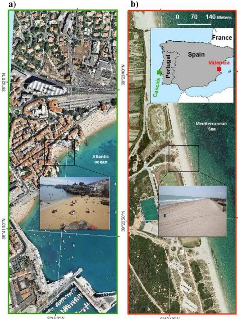
Two very different coastal areas are modelled in this work. The first one (see Figure 1b) is El Saler (Valencia, Mediterranean coast, Spain), a long micro-tidal beach (tide regime changes lowers than 0.18 m) where predominates the low and sandy coast along a wide shoal. The beach segment modeled in this work is about 100 m long. From a geomorphological point of view, this coastal strip has suffered strong erosion problems in the last decades. The erosion is related with sand retention by the jetties of the port of Valencia (north of El Saler beach) which interrupt the littoral drift (Sánchez-García et al., 2015). The second one (Figure 1a) is Praia da Rainha (Cascais, Atlantic coast, Portugal), a mesotidal pocket beach with astronomical tide range between 2 or 3 m. Praia da Rainha is encased by rocky outcrops and baked by artificial structures, and extents about 50 m alongshore.
With regards to the data, high precision measurements were acquired during several field campaigns in order to truly monitor the reliable emerged beach area. The use of Global Positioning Systems in Real-Time Kinematic (RTK-GPS) allows a 3D analysis to characterize coastal changes with accuracies lower than 2 cm in planimetry and within 4 cm in altimetry. The path followed in data collection consists in going over the beach profile in a zig-zag way and from west to east taking a point every two or three meters. Thereby, an average of 15 points each transverse profile is achieved and covering a sandy strip of around 45 m. The planimetric coordinates (XY) and orthometric altitudes (Z) are referenced respectively in the UTM projection and the EGM08.
A set of photographs is taken at dates as most coincident in time as possible with the acquisition of GPS data. Therefore, on the one hand, we have a total of four beach measurements at El Saler beach, covering the spring months since April to June of 2014, specifically the days: 10th April 2014, 19th May 2014, 28th May 2014 and 5th June 2014. Other days also were thought a priori as possible data but finally were barred because the meteorological factors make unable the use of photographs. Thus, according to the data time period, the beach will suffer a
small wave impact designing a characteristic summer beach profile. The sediments are migrating onshore offering a volatile slope which will change its plain profile to another more inclined reaching the 3 m of difference in elevation between the profile endpoints. On the other hand, in Praia da Rainha the field campaign was carried out on 2nd October 2015 at low tide while the beach profile was representative of winter conditions. Therefore, along the 45 m wide beach, the slope reaches the 3.5 m of difference in elevation between the profile endpoints.
In addition, the models might be georeferenced by the location of some available GCPs which can be displayed clearly and unequivocally on the photos. An ideal control point would be a unique element, static and not easily alterable. Moreover, the distribution of them should be well spread out, covering all the study area and located in different elevation planes being its proper establishment one of the most important steps. Nevertheless, the beaches are too homogeneous media, not characterized by having enough unique and unalterable features such as rocks, walls or other elements to use as GCPs and sometimes this fact may hinder the work. In these cases, conspicuous external elements should be provided to bring heterogeneity to the sandy surface. This problem is obvious in El Saler beach where some surveying rods are used as GCP.
Finally, some modeling essays are performed in a hydraulic pilot channel whose size is 4 m long, 0.6 m wide and 0.4 m depth. This work will show again how the SfM is able enough to create a high resolution reconstruction of the sediment on the riverbed before and after some morphological evolution.
Figure 1. Cartography of the evaluation coastal areas. Both sites are marked in the location map (up to the right) by a green and red rectangle respectively in a) and b).
Figure 2. Two different 3D point clouds from El Saler beach which differ depending on the POV and the methodology carried out. The camera positions and the consequent photos are painted by blue rectangles and we appreciate in a) how the photos are taken from the beach, meanwhile in b) are taken from the construction. The right of the Figure shows a photo which has taken part in each one of the left 3D point performance respectively, and being its camera position marked with a red rectangle.
a)
b)
3. METHODOLOGY
Using ground-based photography to achieve digital models by SfM photogrammetry it is known that the first and main important step is the acquisition of a competent set of photos covering the study area. Moreover, the quality of the photos does not matter as much as the way in which they are taken. In fact, the three assessments presented in this work, use simple and non-metric digital cameras such as a Kodak Easyshare M863 in El Saler beach, a Pentax Ricoh WG-3 in Praia da Rainha and a Canon EOS 400D for the hydraulic pilot channel. Using them, the zoom lens is fixed to the infinity and taking care that the photos do not blur. The correct and uniform overlap about the 60% between adjacent photos is achieved adopting short camera baselines and never neglecting the convergence of shots. Furthermore, it is compulsory assure that each captured feature appears at least in five different photos. These considerations are common for the three study sites while the procedure of capturing photos is refined depending on the morphology and characteristics in each area. The resulting set of photos should cover the whole area of interest and avoid useless information that would add noise.
In El Saler beach, we implement two different methodologies of taking photos (see Figure 2) depending on the point of view (POV). The first one consists in locates the camera from the beach (camera elevation around the zero mean sea level), meanwhile in the second, the camera will be located from an existent construction about 6 m high next to the shore. Following the first methodology, the camera is pointing landward and moving longshore each half meter where three shots are taken every time: two shots at the head height and not perpendicular to the coastline but introducing a slight turn both left and right, and the third shot covering a central position as high as possible (see Figure 2a). With regards to the second
methodology from the construction, it will require a much lower number of photos to cover the same beach area due to the height difference as Figure 2b shows. Here, the photos are taken by the same procedure but avoiding the third shot from each camera position. Note that for these two first tests, the whole of photos which take part in each model, have the same elevation meanwhile in the study presented below, the photos come from different elevations.
The protocol followed at Praia da Rainha is a bit different adapting the shots to its pocket and encased form (Figure 5 shows these camera positions). Different sets of photos are acquired, always more than five in each one, and taking advantage of the different heights from where the largest beach coverage may be seen. Nevertheless, the camera baseline continues around half meter.
For the channel reconstruction in an indoor laboratory, some tests are carried out to know about the best procedure. It is based on making three passes of photos at different elevations for each side of the channel meanwhile the camera is pointing to the opposite. The idea consists in modifying successively the inclination of the camera. Therefore, a first pass is done with vertical photos taken from the channel height; a second pass, a bit higher, where the photos have a deviation of 40º from the vertical; and the highest last, with photos turned within 80º and pointing almost perpendicular to the riverbed.
photos. Finally, from the point cloud, we obtain a mesh generation and some rendering products as the high accuracy SfM-DEMs analysed in next section.
4. RESULTS
4.1 Assessing the photogrammetric SfM-DEMs from El Saler beach.
According to the previous methodology, we are going to analyse carefully the partial results. Remembering, in this study area, the 3D beach morphology is going to be assessed for four different days and also, each of them, since two different points of view with respect to the shooting process (from the construction and from the beach). Consequently, in this part we manage a whole of eight different kinds of results.
Once all the photos are well aligned and the preliminary simple point cloud is done, the next step is to ensure the accuracy achieved in the 3D point cloud. Then, including the GCPs in the bundle adjustment, we analyse the obtained errors checking their estimated positions in the point cloud against their real ones. These values should range within the GPS accuracies as it
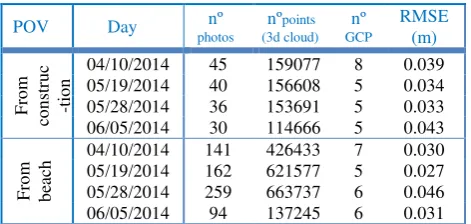
happens in our models having errors between 7 mm and 5.8 cm in the worst case. Furthermore, according to these GCPs errors, the program calculates the setting root mean square error (RMSE) which explains about the quality of the final performance. Then, Table 1 shows the RMSE achieved in the bundle adjustment for each of the eight tests as well as other indicators which describe them.
Results show that RMSE are similar for both methodologies. However, the effort needed is much lower for the first one (see the numerous camera positions in Figure 2a against those in Figure 2b). The time required to take the photos as well as the consequent computing time is reduced and efficient enough. Thus, having an average around 40 photos with a correct overlap and around 5 GCP to georeferenced the model, we achieve a 3D point cloud compound by a whole of 150000 points approximately and a point spacing within 0.27 m. Moreover, the point cloud reaches till 100 m longshore and defines a competent DEM of the beach.
The evaluation of the photogrammetric results is made through the comparison between the SfM-DEM and the GPS data measured at the same day.
±
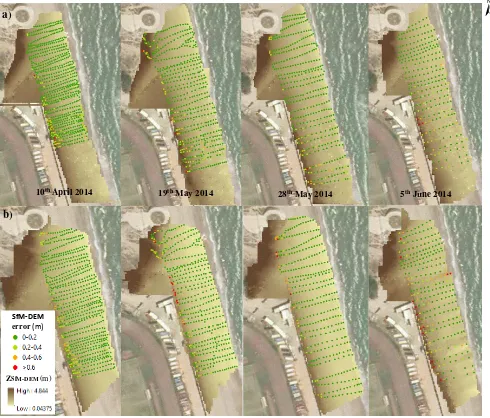
Figure 3. Cartography of the eight SfM-DEMs corresponding to the four studied days and depending on the POV. The results in a) are taken from the construction and in b) from the beach. The DEMs are represented by a brown colour scale which it darkens according to altitude. Moreover, the GPS data are shown by points whose colour indicates the magnitude of the differences in absolute values |ZGPS - ZSfM-DTM| ergo, the SfM-DEM errors.
a)
b)
19th May 2014
10th April 2014
28th May 2014 5th June 2014
SfM-DEM
error (m)
-0,7 -0,6 -0,5 -0,4 -0,3 -0,2 -0,1 00,1 0,2 0,3 0,4 0,5 0,6 0,7 0,8 0,9
Histogram of errors 04/10/2014 Box plot of errors 05/19/2014
0 0.4 4
0.8
-0.4 (m)
Figure 4. Analyses of the distribution errors on 10th April and 19th May of 2014 (both SfM-DEM taken from the construction). Table 1. Indicators showing the way in which the eight tests
have been carried out: the number of photos which takes part in the matching process, the whole of points which form the 3D cloud, the count of GCPs used to achieve the best fitting, and the overall fit error.
Moreover, to avoid errors in the interpolation during the DEM construction, we decide to check each SfM-DEM pixel against each GPS elevation value as Figure 3 describes. This figure shows that the quality of the models measured by the absolute elevation differences (ZGPS - ZSfM-DEM) is generally lower than 20 cm. Another key issue is the spatial pattern of the error distribution. The SfM-DTM works almost perfectly in the entire central part of the beach while the larger errors are concentrated along the beach profile endpoints: (i) biggest errors in the landward border where the beach slope increases, and (ii) many points near the shore with a bigger error than its neighbours. The first type of error (i) can be explained by the way in which these are calculated. The SfM-DEM raster format -1 m resolution- affects to the error magnitude in steeper areas, especially if we consider that the landward end of beach is limited by a wall around 2 m high. The second type of error, that occur near the shore (ii), can be related to the fact that the measured GPS altitudes in wet and soft sand are less accurate, as well as related to the loss of information on the photographs to remain hidden behind the beach berm.
Table 2 summarizes the statistics of the eight tests performed; whose sample size ranges between 254 and 773 elements depending on the number of GPS measurements. Negative values show that generally the SfM-DEM is overestimating the true terrain elevation values. The solvency of all SfM-DEMs is verified because the averages of the differences between GPS and SfM-DEM vary between -5.8 and -12 cm.
POV Day Mean Std. Max Min Table 2. Statistical values in meters of the differences between the SfM-DEMs elevation values and the GPS measurements.
Error analysis also gave insights on their distribution. For example, according to the histogram in Figure 4, we know that the whole of differences on 10th April, data taken from the construction, achieve a mean value of -7.3 cm and its distribution preserves symmetry despite having a more pointed shape than the normal distribution. Furthermore, we perceive how the 50% of those errors are between -1.1 and -1.8 cm. With regards to the box plot showed in the same figure, this is now
representing the error distribution on 19th May, data also taken from the construction. And, once again, the 50% of the errors approach the -1 cm.
4.2. Assessing the photogrammetric SfM-DEMs from Praia da Rainha.
Processing Praia da Rainha data acquired on 2nd October 2015, also allow to get a competent 3D point cloud of this mesotidal pocket beach. Following the methodological protocol, the bundle adjustment is done by using six GCP and a whole number of 47 photographs taken in different sets such as we see in Figure 5. After the photo alignment, the georeferenced point cloud achieves an overall root mean square error within 29 cm. This value is substantially higher than the GPS accuracy, consequence of the GCPs distribution on objects outside the beach area and being sometimes complicated their optimal detection in the photographs. However, the model is good enough to define the beach morphology with high resolution as the results show. The dense point cloud is formed by a whole of almost eleven millions of points spaced each 2.3 cm and covering all the intertidal and supratidal beach areas.
In addition, the resulting SfM-DEM is compared with six GPS profiles measured cross-shore (a total number of 70 GPS data values listed in Fig. 6). Both data (SfM-DEM and GPS) should be able to recreate the beach morphology in a similar way despite the intrinsic disparities in accuracy. Analysing statistically the differences between the elevation values, we achieve the results shown in Table 3.
Table 3. Statistical values in meters of the differences between the SfM-DEMs elevation values and the GPS measurements.
Finally, Figure 7 shows in each different profile how the beach face slope is defined according to both data. We realise that the SfM-DEM values design the beach profiles in the same way as the GPS measurements although underestimating them in a range from 12 cm landward to 38 cm near the shore.
In this regard, we are able to guarantee that an elevation model obtained by photogrammetry is able to describe the beach morphology with a precision that matches the one that would be obtained by a GPS survey. To reach this conclusion has been important taking care about the proximity of photogrammetric and GPS data, ensuring that both sets of data provide information of similar punctual time values.
4.3. Application of SfM photogrammetry in a pilot channel.
The previous sections have proved the potential that the SfM photogrammetry has to recreate efficiently the beach area. Nevertheless, these techniques also can be applied to monitor other dynamic environmental areas.
One of the most immediate applications of SfM photogrammetry is the analysis of morphological changes because having elevation models for different days is easy measure the magnitude of changes. In this section we show how the photogrammetric models can describe extremely well the sedimentary movements in a riverbed. The experiment is done in a pilot channel with a constant water flow where it aims to know the impact suffered by the sediments as a result of the construction of a bridge. Thus, it is created a SfM-DEM before any water flow proceeds through it, and another one after it. However, to achieve the best point cloud results, in both cases the channel had to be completely dry (emptying water) and taking care not to alter the shape of the sediments.
Following a good methodology to take the photos, the SfM technique is able to localize the camera positions and to solve the scene geometry. In these examples, a total number of 76 photos are used to achieve the redundant bundle adjustment based on matching features and thanks to the overlap between photos. The final 3D dense point clouds are about 690000 points spaced each 1 mm approximately. Moreover, the model is georeferenced in a relative coordinate system by six control points. These points are located in the side walls of the channel and measured with a flexible tape.
Figure 5. Dense point cloud and 3D reconstruction of Praia da Rainha. The blue rectangles represent the cameras taken by sets of photos from different positions.
Figure 6. Cartography of Praia da Rainha SfM-DEMs. The DEM is painted by a colour scale according to altitude. The GPS data are shown by points whose colour indicates the magnitude of the differences |ZGPS - ZSfM-DTM| in absolute values; ergo the SfM-DEM errors.
SfM-DEM error (m)
ZSfM-DEM (m)
PR-1
1 13
14
23
24
35 36
51
PR-4
PR-5
62
52
70 63
PR-6
PR-2
Figure 9. Representation of the differences between the SfM-DEMs shown in Figure 8.
Figure 8. Orthogonal view of the channel 3D model at two different times.
a)
b)
Therefore, the accuracy might range around a few centimeters and in fact, the overall RMSE is 4.1 cm.
After a careful treatment of both 3D point clouds, Figure 8 shows the models before and after the water flow experiment was carried out. Despite the good results, it is important to comment the difficulties had with the first model (Figure 8a). These are consequence of the excessive uniformity in the photos, without practically homologous entities to recognize. Thus, the software has problems to locate the cameras in the correct place. The solution is to work with two models, one for each half of the channel, and then joining both. However, in Figure 8b, the different shapes created in the sediment by the water flow help in the correlation process.
Subtracting both georeferenced SfM-DEMs we obtain the magnitudes of morphological change in relation to sediment transport (see Figure 9) which range between almost 0 (sand motionless) and 4.47 cm. Moreover, we realise that the sediment of the riverbed is following the expected behaviour relative to the channel amplitude and the water velocity. Considering that the water flows from left to right, the sediment is undermined where the channel becomes narrower next to the bridge brackets (with losses within 4.47 cm), and it is accumulated just behind them, forming mounds of sediment up to 3 cm. Additionally, these values have been successfully validated with some accurate measurements done in laboratory.
5. CONCLUSION
The systematic monitoring of some natural phenomena knowing its dynamism and behaviour is a need in the context of good management of natural resources. The understanding of changes
ZGPS (m)
ZSfM-DEM (m)
and actions through a retrospective view help to have an overview for subsequent predictions and future actions avoiding unwanted coming situations.
Working at low spatial scales and having into account that a high repeatability is a strong point in the monitoring of any event - for example the tracking of extreme storm events or close range monitoring-, the methodology carried out in this work is a good option to follow in the study of natural changes because its low cost, usefulness and few technical requirements. Two main goals have been developed in this paper:
i) Resulting SfM-DEMs obtained for several days and in two different study areas, prove the photogrammetry skills for coastal purposes. The differences range around an average of 6 and 12 cm for the whole of profiles along the Spanish microtidal beach and, within 25 cm in the Portuguese mesotidal beach. These errors are in line with the success got along the methodological process (GCP definition, camera positioning and the bundle adjustment).
ii) On the other hand, the application of the SfM to measure sedimentary changes in fluvial systems. Again the results explained the sedimentary dynamics occurred in the riverbed and the photogrammetry overcomes other harder and more expensive techniques.
However, and despite the large benefits of the SfM photogrammetry, we want to remark the importance of conducting a careful methodological protocol especially in the process of taking photographs to achieve a good 3D model. The excessive uniformity found in environments such as beaches or riverbeds requires a systematic overlapping between photos and a brainy procedure in the positioning and orientation of the cameras.
The culmination of a study as here presented, contains its full potential and practical use in the monitoring of confined spaces that allow the subsequent prediction of future situations. Reach something as tangible as the mapping of a coming situation, will help in the sustainable planning of the natural resources. New the Spanish Ministry of Economy and Competitiveness called CGL2015-69906-R and other of the Valencia Regional Government called AICO/2015/098. The authors are grateful to Jesús Vaquero for the collaboration during his Bachelor's Degree project and to Mafalda Carapuço for her contribution to the Portuguese field work.
REFERENCES
AgiSoft, 2014. AgiSoft PhotoScan professional edition. http://www.agisoft.ru/products/photoscan/.
Almonacid-Caballer, J., Sánchez-García, E., Pardo-Pascual, J.E., Balaguer-Beser, A., Palomar-Vázquez, J., 2016. Evaluation of annual mean shoreline position deduced from
Landsat imagery as a mid-term coastal evolution indicator. Mar. Geol. 372, pp. 79–88. doi:10.1016/j.margeo.2015.12.015.
Gonçalves, J.A., Henriques, R., 2015. UAV photogrammetry for topographic monitoring of coastal areas. ISPRS J. Photogramm. Remote Sens., 104, pp. 101–111. doi:10.1016/j.isprsjprs.2015.02.009.
Hugenholtz, C.H., Whitehead, K., Brown, O.W., Barchyn, T.E., Moorman, B.J., LeClair, A., Riddell, K., Hamilton, T., 2013. Geomorphological mapping with a small unmanned aircraft system (sUAS): Feature detection and accuracy assessment of a photogrammetrically-derived digital terrain model.
Geomorphology, 194, pp. 16–24.
doi:10.1016/j.geomorph.2013.03.023.
James, M.R., Ilic, S., Ruzic, I., 2013. Measuring 3D coastal change with a digital camera. Coastal Dynamics, pp. 893–904.
Javernick, L., Brasington, J., Caruso, B., 2014. Modeling the topography of shallow braided rivers using Structure-from-Motion photogrammetry. Geomorphology, 213, pp. 166–182. doi:10.1016/j.geomorph.2014.01.006.
Nácher-Rodríguez, B., Vallés-Morán, F.J., Balaguer-Beser, A., Capilla, M.T., 2015. Numerical-Experimental Modelling of Local Scouring Downstream of Protected Bridges in Alluvial River Beds. E-proceedings 36th IAHR World Congr., pp. 1–12.
Pikelj, K., Ilić, S., James, M.R., Kordić, B., 2015. Application of SfM photogrammetry for morphological changes on gravel beaches: Dugi Rat case study (Croatia). Conférence Méditerranéenne Côtière Marit. Ed. 3, Ferrara, Ital., pp. 67–72.
Ružić, I., Marović, I., Benac, Č., Ilić, S., 2014. Coastal cliff geometry derived from structure-from-motion photogrammetry at Stara Baška, Krk Island, Croatia. Geo-Marine Lett., 34, pp. 555–565. doi:10.1007/s00367-014-0380-4.
Sánchez-García, E., Pardo-Pascual, J.E., Balaguer-Beser, A., Almonacid-Caballer, J., 2015. Analysis of the shoreline position extracted from Landsat TM and ETM+ imagery. In: The International Archives of the Photogrammetry, Remote Sensing and Spatial Information Sciences - ISPRS Archives, Vol. 40, pp. 991–998. doi:10.5194/isprsarchives-XL-7-W3-991-2015.
Uunk, L., Wijnberg, K.M., Morelissen, R., 2010. Automated mapping of the intertidal beach bathymetry from video images.
Coast. Eng. 57, pp. 461–469.
doi:10.1016/j.coastaleng.2009.12.002