A DYNAMIC THRESHOLD CLOUD DETECTING APPROACH BASED ON THE
BRIGHTNESS TEMPERATURE FROM FY-2 VISSR DATA
X. Daxiang a, *, T. Debao a, W. Xiongfei a, W. Qiao b
a Changjiang River Scientific Research Institute, Changjiang River Water Resources Commission, Wuhan, China – [email protected], [email protected], [email protected]
b Network and Information Center, Changjiang River Water Resources Commission, Wuhan, China – [email protected]
THEME: DATA – Data and information systems and spatial data infrastructure.
KEY WORDS: Cloud detecting, Brightness temperature, FY-2 VISSR data, Dynamic threshold, Temporal-Spatial scale
ABSTRACT:
The traditional statistical methods and radiation transfer theory methods for cloud detecting have a high adaptability just only in those areas with a uniform surface coverage and noncomplex terrain. Therefore, adapted to large spatial and temporal scales, in this work a cloud detection method is developed, seeking the main influencing factors of the change of Brightness Temperature(BT) of clear sky and their relationships, researching the change regularity and normal fluctuation range of BT on the basis of function fitting, setting the cloud detecting dynamic threshold depending on the cloud spectral characteristics, and making accuracy assessment in order to ensure higher adaptability and accuracy of this cloud detecting method. In this paper, a dynamic threshold algorithm is presented for cloud detection using daytime imagery from the VISSR sensor on board FY-2C/D/E, which is the first generation geostationary satellite. And the land surface/brightness temperature influence functions are analysis and established, including latitude, longitude, altitude, time, land cover. The theoretical temperature value of clear sky can be calculated through these influence functions. Then, the dynamic threshold cloud detection model is proposed based on the high temporal resolution of VISSR data. Meanwhile, the land surface emissivity is considered as the main factor to the change range of brightness temperature which determines the dynamic threshold for cloud detection. Finally, the dynamic threshold cloud detecting model is evaluated using FY-2C/D/E VISSR data covering China, and the Kappa of dynamic method is maximum, equalling 0.6195, which is much higher than the indexes for the reflectivity and BT fixed methods, equalling 0.4511 and 0.403, respectively. Consequently, the dynamic threshold cloud detecting method provides an important improvement because the spatial, temporal and geographic characteristics were considered into the model.
* Corresponding author. Email:[email protected]. 1. INTRODUCTION
1.1 Background
Clouds present a variety of shapes and sizes, covering, at any time, more than 50% of the Earth surface (Saunders, et al., 1988). According to the height from cloud bottom to the ground, clouds have been traditionally classified into three types: high, middle and low cloud. But their radiation properties, and thus their influence on the radiation balance of the Earth-atmosphere system, not only depends on their altitude but also on their optical thickness or the size of their particles, which can be water droplets or ice crystals (Hunt, 1973; Kokhanovsky, et al., 2006).
Remote sensing technique is undoubtedly becoming a crucial approach to provide these observational facts for both the cloud detection and the model verification. Cloud detection techniques from remote sensing imagery can be roughly classified in three main categories (Goodman, et al., 1988): threshold methods, statistical approximations and those techniques based in radiation transfer computations. The first type of method is based on the adequate selection of thresholds in the different spectral bands to distinguish cloudy pixels from clear ones. These thresholds can be also applied to a combination of spectral bands or to new variables obtained from them, such as some measurements related to the space consistency and phase correlation. Typical examples of these techniques include the International Satellite Cloud
Climatology Project (ISCCP) and the NOAA Cloud Advanced Very High Resolution Radiometer (CLAVR) (Murtagh, et al., 2003). The statistical methods include histogram, clustering and other image processing models analyses, for instance, the AVHRR Processing scheme over cloud Land and Ocean (APOLLO). The radiation transfer technology methods mainly consider remote sensing imaging mechanism and land surface covers’ spectral features in different channels (Bao, 2008). With the development of cloud detecting field, some breakthroughs were reached in recent years using new approximations, such as, artificial neural network, expert systems, fractal texture and spatial structure analysis, and so on. Simpsona et al. (1995) improved the threshold method in a cloud detecting technique over ocean surfaces. Karner et al. (2001) proposed the 5D Histogram Techniques method based on spectral characteristics of clouds. Chen et al. (2003) considered the fractal texture as an important factor for cloud detecting. Song et al. (2003) studied an auto-detecting algorithm on the basis of spatial structure analysis and neural network. Choi et al. (2004) implemented cloud detection for the Landsat images through combining the superiority of threshold and shadow matching.
of model derivation. Therefore, adapted to large spatial and temporal scales, in this work a cloud detection method is developed, seeking the main influencing factors of the change of BT of clear sky and their relationships, researching the change regularity and normal fluctuation range of BT on the basis of function fitting, setting the cloud detecting dynamic threshold depending on the cloud spectral characteristics, and making accuracy assessment in order to ensure higher adaptability and accuracy of this cloud detecting method. 1.2 Existing Methods
The cloud detection method for the data of geostationary orbit meteorological satellites (such as FY, GOES, GMS, MTSAT series) have greatly development in the last few years (Ellrod, 1995; Lee, et al., 1997; Ahn, et al., 2003). A bi-channel dynamic threshold algorithm is used to identify clouds on GMS-5 images (Liu, et al., 2005). The threshold values of clouds and surface objects are gained in visible and infrared window channels by means of a statistic histogram analysis. The multi-channel cloud detection algorithms established with the data of GMS-5, including two infrared split channels, visual channel and water vapour channel (Ma, et al., 2007). The experiments proved that the cloud detection threshold values are changing with the season, solar altitude and latitude. Similarly, the channel combination methods of cloud detection are used to MTSAT and FY-2 data (Gao, et al., 2009; Liu, et al., 2011). Based on the highly temporal resolution of the geostationary orbit meteorological satellite, the brightness temperature or temperature time series imageries can be utilized in the cloud detection of nominal imageries, and in identifying clouds that are developing rapidly or located at the boundaries of the moving clouds (Yang, et al., 2008).
2. STUDY AREA AND DATA
The study was conducted in the whole land of China, with latitude ranging from 4ºN to 53ºN and longitude ranging from 73ºE to 135ºE, respectively. This large region comprises of various kinds of landscapes.
FY-2C/D/E is the first generation of operational geostationary orbit meteorological satellite in China, C / E star (E star is the successor of C star) is positioned at 105 degrees east longitude and D star is positioned above the equator in 86.5 degrees. VISSR (Visible and Infrared Spin Scan Radiometer) is the major load of FY-2 series, including a visible channel (0.55-0.90µm, 1.25 kilometre spatial resolution) and four infrared channels (10.3-11.3µm、11.5-12.5µm、6.3-7.6µm、
3.5-4.0µm, 5 kilometre spatial resolution). The temporal resolution of the sensor reaches one hour in normal pattern and half hour in flood season pattern severally. VISSR can obtain daylight image of visible light band, day and night IR images in a water vapour absorption band. It can be used to collect data for meteorological, oceanographic, hydrological and other applications (Dong, 2008). The FY-2C/D/E VISSR data used in this article were provided by the China Meteorological Administration.
3. METHOD
3.1 Theory
When clouds are observed by radiometers on-board satellites, they present a relatively high reflectivity in the visible and near-infrared bands and low Brightness Temperatures (BT) in the thermal infrared bands (Peak, et al., 1994). Around 0.936um band, with the impact of the absorption by water vapour, the
clouds reflectance is on the absorption valley. Owing to the similarity in the spectral characteristics between Ice clouds in the high family of clouds (i.e. cirrus) and snow, the two is not easy to be distinguished. In 1.38um mid-infrared channel, due to the strong absorption of the radiation by water vapour, the radiation from low, middle cloud and ground is difficult to reach the sensor, the ground reflectance is almost zero, while the cirrus clouds ,which is the high family of clouds, have small humidity and high reflectivity. In many cases, cloud detection using remote sensing is mainly achieved by setting the appropriate thresholds on the basis of the clouds characteristics of high reflectivity and low BT.
However, the use of fixed or semi-fixed thresholds to implement cloud detection methods is only possible when they are applied to a small area. So an adaptive threshold cloud detection method is necessary to improve cloud detection accuracy in large territories or at a global scale.
3.2 Clear Sky Brightness Temperature Calculated Model
Land Surface Temperature (LST), which is an important climatic factor, not only depends on the effectiveness of the surface to absorb solar radiation, but also on the thermal properties of land surface, including surface type, moisture conditions and heat balance(Becker, et al., 1990;Campbell, 2002). Remote sensing image cloud detection is usually conducted by setting the corresponding thresholds based on the two cloud characteristics of high reflectivity and low brightness temperature, but these two factors change with different environment under different time and space conditions. As a result, it is difficult to use a relatively fixed threshold to obtain accurate cloud detection results. However, according to the solar radiation model, the surface temperature of completely clear sky pixels changes regularly, and these changes can be estimated. So, on the basis that the temperature of certain pixel is lower when it is covered by cloud, automatic threshold for cloud detection can be achieved by seeking normal range of each pixel’s surface temperature.
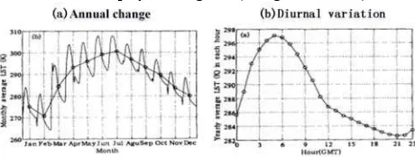
According to the research on inter-annual variation of solar radiation, LST has the same tendency in different seasons (Song, et al., 1993). Therefore, eliminating some uncertainty, LST can be determined by the total solar irradiance. The annual change and diurnal variation of clear sky LST, in the region of East Asia in 2000 is displayed in Figure 1(Wang, et al., 2005).
Figure 1. Change of clear sky LST in 2000, in East Asia Figure 1(b) shows that, with the impact of solar radiation, the gradient of surface temperature change during daytime is much larger than that at night. For the region of East Asia, surface temperature rapidly increases after GMT 0:00 and reaches the maximum at GMT 5:00, then the temperature experiences a rapid drop and reaches the minimum at GMT 21:00. Obviously, the gradients of the two stages are different as a result of solar radiation. A large number of experiments confirm that, anywhere, the LST have a similar behaviour, however, the position of peak and valley will move with the change of temporal and spatial conditions.
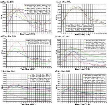
several BT curves that describe the BT 24-hour change of clear sky pixels obtained from FY-2C/D/E VISSR data in a variety of conditions (time, location, land cover, elevation):
Figure 2. Temperature change curves in China area: day is the date, lon is the longitude, lat is the latitude, dem is the elevation above sea level and lc is the land cover type as defined in IGBP,
and the unit if dem is meter
As shown in figure 2(a) the curve maximum moves left, the time point when temperature reaches maximum value during the day move forward. Because, on the basis that the sun rises in the east and sets in the west, the greater longitude is, the sooner the temperature reaches the highest point. Accordingly, the time when the temperature gets the maximum value is related to the longitude. In addition, the figure also demonstrates that the elevation, to a great extent, affect the mean temperature and temperature difference, which are the amplitude and intercept in the figure, respectively. How the temperature is affected by elevation is analysed in detail below. The change trends in Figure 2(b) are the same as in Figure 2(a) that reflect the relationship in the temperature maximum and longitude. The three curves in Figure 2(c) confirm that the elevation does impact on the temperature changes. In Figure 2(d) it can be observed that the longitude and other factors show the same effect on the temperature curve: the blue line and green line, and the deep red as the longitude difference between, leading to the moment the temperature reaches its maximum biased shift. Because the reasons for seasonal changes, Figure 2(e) show that the winter temperatures have a diurnal variability smaller than in Figure 2(a), (b). At the same time, differences in land cover types which largely determine the temperature difference is shown in Figure 2(e). Figure 2(f) shows the dependence of the temperature curves on the latitude, showing a negative correlation between latitude and temperature.
From the above explained analysis, we can conclude that brightness temperature of clear sky pixels are related with longitude, latitude, elevation, season, the time of day, land cover type and other factors. It can be seen from Figure 2 that the curve that describes the temperature change of each pixel throughout the day are smooth and regular (the curves of sparse cloud-covered pixels have a little oscillation). The shapes of the curves are similar to a parabola and trigonometric functions plots. In this study, for the cyclical change of temperature and solar radiation prototype model taken into consideration,
trigonometric function was selected to calculate brightness temperature of clear sky pixels.
The theoretical value of brightness temperature under clear sky conditions can be calculated by constructing functions based on the relationship between brightness temperature and the longitude, latitude, elevation, season, the time of day and land cover type. In general, we can observe that: (1) In the same position, where the geographic information, terrain and land cover are fixed, daily and annual variation of brightness temperature under clear sky occur, respectively, with time of day and with the season of the year. (2) For the same time, the brightness temperature, under clear sky conditions, changes with the position as well as the terrain and land cover. Therefore, the brightness temperature for clear pixels can be expressed as an abstract equation:
(
,
, , ,
, )
p
BT
=
f lon lat d t dem lc
(1)Where
BT
p is the theoretical value of brightness temperature,f is the function to calculate brightness temperature.
The development of the general model to estimate the BT is explained in the next subsections.
3.2.1 General Model: There are two temperature change cycles: a short-term temperature change accounting for the cycle of day and night, and a long-term temperature change, an annual cycle of seasonal changes. Therefore, this article intends to study short-term temperature changes to determine the function of the cycle of 24 hours, taking into account that this work is focused on the cloud detection during daytime. The first half of the curve in Figure 1(b), which corresponds to daytime temperatures, can be approximated by equation (2) expression:
1sin[ ( 1)] 1 0 12 12
p
BT =a
π
t−b +cLL ≤ <t (2)Where a, b and c are the curve coefficients, mainly influenced by longitude, latitude, elevation and land cover, and t is GMT time of day. Because the FY-2 VISSR cover the Asia-Pacific area, the variable t was selected between 0 to 12 of GMT, directing the day time of China, in this study.
3.2.2 Longitude Influence Function: Each satellite image have its own explicit acquisition time, however, satellite images have a larger coverage area. Because of the relationship of local time and longitude, the imaging time only corresponds some image point’s local time, named Main Points (MP). In order to eliminate the difference from different longitude, we can obtain every points imaging local time through the relative position between these points and MP. Generally, the local time becomes later with longitude from west to east in the eastern hemisphere, concretely, one hour of local time difference corresponds to 15 degrees of change in longitude. Thus, the time difference can be calculated by:
(
MP) /15
t
lon lon
Δ =
−
(3)Where
Δ
t
is the time difference between every point and MP,lon
is longitude of every point,lon
MP is longitude of MP. Based on these analyses, in Figure 1(b), the first trigonometric function reaches the peak at GMT 5:00 in the East Asia area. The peak definition of the trigonometric function can be expressed:1_ 1 1 6 5
15 4 15
MP MP
pv
lon lon T lon lon
t = +b − + = +b − + = (4)
Where
t
1_pv is the peak of trigonometric function and T is theperiod (24 hours).
Equation (4) can be conducted to equation (5):
1 1 ( MP) /15
Finally, the general model can be rewritten using the following
3.2.3 Latitude Influence Function: The external energy from solar radiation is one of the primary energy sources to create the ecosystem differences. The primary control of climate at the global level is variation in solar energy, which is related to latitude. The amount of solar radiation generally decreases from the equator to poles, partly due to increases in the angle of incidence of the atmosphere. As a result, LST is reducing with the latitude increasing, which has two reasons: (1) Solar radiation angle increasing; (2) Atmosphere effective thickness changing. As illustrated in Figure 3, for the same solar radiation, the received amount per unit area in low latitudes is larger than in high-latitude areas.
Figure 3. The relationship between solar radiation and solar radiation angle
To simplify the latitude influence function, in this work only considers the impact of solar radiation angle is considered. Let’s assume that two beams of sunlight, squares of side length L and parallels to the equatorial plane, shine on the two
latitudes
ϕ
1 ,ϕ
2 , respectively. As in Figure 3(b), in thelatitude plane, the Earth radius and its projection line defines a right triangle. Based on the geometry relationship of triangles, the vertical height of the bottom and top of the sunlight can be calculated by:
On the basis of this assumption, the difference of the bottom and top of the sunlight is just the height of sunlight, as in equation (8):
_ _
T L
H ϕ−H ϕ=L (8)
Similarly, equation (9) can be derived:
1 1 1
Δ
are central angles, which are close to zero, caused by the height of sunlight. From equation (9):1 1 1 2 2 2
sin(ϕ + Δ −ϕ) sinϕ =sin(ϕ + Δϕ) sin− ϕ (10)
Based on product to sum equation, equation (10) can be derived:
1 1 1 1 1 The arc of a sector can be calculated by the following:
s s s
l =r
θ
(13)Where
l
s is the arc of the sector,r
sis the radius of the sectorand
θ
s is its central angle.The ratio of the solar radiation received in different latitudes can be calculated by:
1 2 2
l
ϕ are the solar radiation, shining areaand arc length of the sunlight beam of the latitude
ϕ
i.Therefore, the latitude influence function can be simplified as the following equation:
2
[cos(
)]
p
BT
=
a
lat
+
b
(15)Where a, b are regression coefficients.
3.2.4 Seasonal Influence Function: Obviously, LST expresses a cyclical change with the seasons (Bailey, 1996). Because the research in this area has matured until now, some statistical experiments are used to verify the seasonal influence function in this paper, as shown in Figure 4:
Figure 4. The regression curves of temperature change in 2006
Based on the brightness temperature series data of the whole 2006 from FY-2C VISSR, in figure 4, the evolution of BT follows a parabolic curve with the season and the symmetry axis is approximately 190 days, which corresponds to late July. Because the parabolic curves have same shapes, the seasonal influence function can be rewritten as one simple equation. However, the y coordinates of the vertex show an obvious fluctuation with the change of location and land cover. It is worth mentioning that this coefficient can be easily obtained from a sum function. Consequently, the seasonal influence function can be approximated by the following equation:
2
0.001526
0.58
p
BT
= −
d
+
d
+
a
(16)Where a is the y coordinate of the parabola vertex.
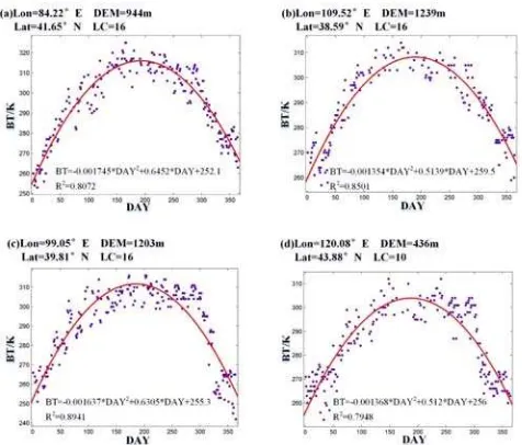
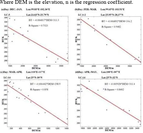
3.2.5 Elevation Influence Function: Elevation changes have a direct effect on temperature. An essential feature of mountainous regions is a vertical differentiation of climate and vegetation based on the effects of elevation change. At an altitude of 8km, the density of the atmosphere is less than one-half its density at sea level.
and a decrease in diurnal variability of temperature with elevation decreasing (Bailey, 1996). Average temperatures drop by about 6.50ºC per 1km However, this rate of decrease is not uniform. Temperatures decrease from the equator toward the poles. The elevation influence function can be drawn as the following equation:
0.0065* p
BT = − DEM+n (17)
Where DEM is the elevation, n is the regression coefficient.
Figure 5. The relationship between BT and elevation
Four groups of FY-2 VISSR data from 2006 to 2011 are selected to plot the regression curves shown in Figure 5, which to verify the elevation influence function. In order to make sure the invariance of the group data, the each dataset have a range of latitude and longitude lower than 7 degrees, and a range of days shorter than 20 days, and a range of albedo lower than 0.05, and have the same land cover types. From this figure, we can find that the experiment results of statistical data are very close to the theory result, and the average correlation coefficient reaches 0.85 based on these statistical data.
Finally, based on the longitude, latitude, seasonal and elevation influence functions and the criterion of building multi-factor model, clear sky brightness temperature can be calculated by:
2
3.2.6 Determining a Dynamic Threshold: In the same solar radiation conditions, the absorption and release heat capacities of different land surface cover types are difference because of their different emissivity. So, their surface temperature is different because their rates of temperature increase and decrease are inconsistent. Therefore, emissivity is one of the main factors that affect the rate of temperature change. Emissivity is the radiated power ratio between actual object and the blackbody with the same temperature, the definition of emissivity is drawn as equation (19):
'/
W W
ε =
(19) WhereW
'
is the object radiant flux,ε
is object emissivity, W is the blackbody radiant flux.Land surface emissivity mainly depends on the material structure and on the spectral bands of the sensor. Qin et al. (2004) considered that the earth surface consists of water, town and natural surface in satellite image pixel scale. The natural surface, which is the most important element, was mainly constituted by natural land surface, woodland and farmland.
The satellite image pixels can be simply considered as mixed pixels which are composed by different proportions of vegetation and bare soil. Thus, the emissivity of a satellite image pixel can be calculated by:
, , , (1 )
i pixel i vFVC i g FVC d i
ε =ε +ε − + ε (20) Where
ε
i v, is the emissivity of vegetation in radiometerchannel i,
ε
i g, is the emissivity of bare soil in channel i andi
d
ε
is the emissivity of channel i because of multiple reflection. As the resolution of the satellite images are very low,the multiple reflection is thought no exist, that is to say,
d
ε
i=0. Finally, FVC is the vegetation coverage, which can be drawn as:
Where
NDVI
S is the typical Normalized Difference Vegetation Index (NDVI) value of pure bare soil pixel, thevalue has been fixed to 0.05 in this paper,
NDVI
V is the typical NDVI value of pure vegetation pixel.Some authors find that the range of emissivity in wavelength from 8µm to 14µm is small (Labed, et al., 1991; Salisbury, et al., 1992; Sobrino, et al., 2001; Mao, 2007). Based on the vegetation classification of International Geosphere-Biosphere
Plan (IGBP), this paper use the research results of
ε
i v, ,ε
i g, ,V
NDVI
andNDVI
S in wavelength from 10µm to 12µm with referencing the channel characteristics of FY-2 VISSR (Rubio, et al., 1997;Zeng, et al., 2000). Therefore, the emissivity can be calculated by the above derivation with the information of land cover classification.The Stefan-Boltzmann Law can be drawn from the Planck equation as the following:
4
W
=
σ
T
(22) Where W is radiation, σ = 5.67*10-8[W•m-2•K-4], T is the absolute temperature of black body.The objects can be classified into two types, selective radiator and grey body, on the basis of the spectral emissivity change pattern with wavelength. Meanwhile, most objects can be seen as grey body. The emissivity equation can be derived:
4
'
W
=
ε
W
=
εσ
T
(23) The blackbody radiation temperature can be considered as the grey body equivalent blackbody temperature, and the relationship of equivalent temperature and object actual temperature can be drawn by the following equation (24):4
= '
T
ε
T (24) From the above equation, the actual object temperature shows an inverse relationship with its emissivity when the spectral radiation is constant.Therefore, the range of temperature change, which will be considered as the dynamic threshold for cloud detection, can be derived by the surface emissivity as:
4 4
4 4
max min max ' min ' ( max min) '
T T T ε T ε T ε ε T
Δ = − = − = − (25)
Figure 6. The dynamic threshold
Therefore, the brightness temperature dynamic threshold model was built using the following equation:
( , , , , , ) ( )
DT p
T =BT − Δ =T f lon lat d t dem lc − ΔT lc (26)
Where
T
DT is the BT dynamic threshold,Δ
T
is the range ofBT in normal conditions,
lc
is the land cover.4. EXPERIMENT AND ANALYSIS
4.1 Dynamic Threshold Cloud Detection
Based on the clear sky brightness temperature equation calculated in previous sections, a collection of 600 groups of data taken in different season, time, longitude, latitude and elevation conditions were used to obtain the model fitting. Table 1 summarizes the regression coefficients on the basis of least squares theory, and the relationship coefficient of regression reaches to 0.8167 based on five years FY-2 VISSR data.
coefficient 0<t<=12
a 19.616
b 50.943
c 0.741
d 0.312
e 230.07
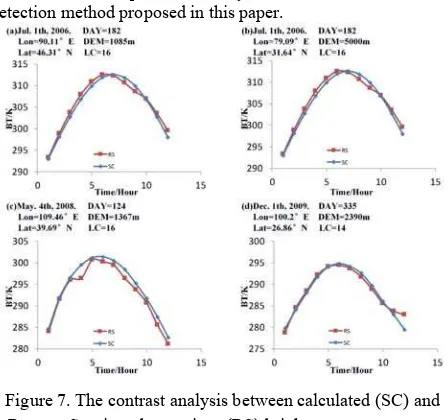
Table 1. Regression coefficients of clear brightness temperature Figure 7 shows the contrast plots between the calculated clear sky BT using the proposed model and the corresponding remote sensing data at the same conditions, such as, longitude, latitude, elevation and date. It can be appreciated that the degree of coincidence of calculated and observed temperatures is very high from 0:00 to 12:00 and the difference is less than 1K. The reason of existing differences is likely due to the fact that in some cases there is not pure clear sky when remote sensing observations were taken. The magnitude of the difference is lower than the expected uncertainty due to sensor noise. In addition, the relatively peak positions between calculated and observed have small offset because of the difference of satellite position and local time of image main points. Figure 8 shows some examples on the BT maps estimated through the proposed model in the most of China area (same as below).
In Figure 8, the change pattern of clear sky brightness temperature with longitude, latitude, season and elevation is evident. From south to north, the BT decreases with the latitude increasing. And the BT values do not change in the longitude direction. The seasonal and elevation influence function plays an important role in the calculated model. Based on the analysis of remote sensing data, the calculated brightness temperature
data have the required accuracy to be used in the cloud detection method proposed in this paper.
Figure 7. The contrast analysis between calculated (SC) and Remote Sensing observations (RS) brightness temperatures
Figure 8. The calculated result of clear sky BT about the Chinese mainland areas
As previously explained, the BT variability can be obtained by the clear sky brightness temperature calculated value and the surface emissivity range of different land cover. Based on the characteristic of low brightness temperature of clouds, the minimum of BT range is considered as the dynamic threshold for cloud detection.
4.2 Analysis of Cloud Detection Results
Two fixed threshold methods based on brightness temperature and reflectivity were used in order to verify the accuracy of the dynamic threshold model in this paper. The two cloud detection methods can be applied to large spatial and temporal scales respectively. The thermal infrared channel was used in the fixed threshold method of brightness temperature, and the visible channels in the reflectivity method. Because the study area is large, the two fixed methods were improved by using regional fixed thresholds based on the classification of land cover. The results of the proposed cloud detection algorithm are shown in Figure 9 for an example image, acquired 20th November, 2010, at 4:15 am. The results obtained using the fixed threshold methods, the original image (visible channel), the computed clear sky brightness temperatures, and the results provided by MODIS algorithms have been also presented.
The fixed threshold cloud detecting methods have relatively low accuracy for the reason that the brightness temperature and reflectivity are highly variable across the study area, which is very vast and contains a great variety of land. Therefore, in this paper, some different fixed thresholds are used in different zones, which have been divided attending to zone characteristics and land covers. Using this approximation, the detecting results have greatly improved, compared to those obtained by the single fixed threshold methods. However, in figure 9, the fixed threshold method that uses the visible channel provides false positive cloudy pixels in northeast and southwest of China (Figure 9(b)). At the same time, the fixed threshold method using the brightness temperature also present an excessive cloud cover estimation in north of China (Figure 9(c)) through visual interpretation. Meanwhile, the fixed threshold is not able to detect thin cloud areas, like in the southeast of China (Figure 9(c)).
Figure 9. Result of cloud detecting (the light is cloud) The temporal and spatial factors, such as, longitude, latitude, season, time and elevation, have been discussed previously in the derivation of the dynamic threshold cloud detecting method. The characteristics of the different areas are obviously reflected in the result of the computed BT (Figure 9(d)). Furthermore, the dynamic threshold is determined by the normal change range of BT based on the land cover information. The detecting accuracy has greatly improved using the dynamic threshold, especially in the thin cloud zones and the transition areas between the cloud and clear sky (Figure 9(e)).
The MODIS cloud product combines infrared and visible techniques to determine both physical and radiation cloud properties (King, et al., 1997; Menzel, et al., 2010). In this paper, the accuracy of dynamic threshold method has been evaluated using the cloud mask provided by MODIS operational products.
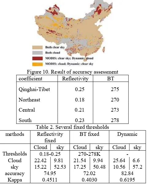
In Figure10, the grey pixels indicate that the reference pixels have been detected as cloud covered by both, MODIS and the dynamic threshold method. The tan pixels indicate that they are clear sky pixels for both algorithms. Meanwhile, the orange pixels mean that the reference pixels have been detected as clear sky by MODIS and the proposed method considers them as cloud covered. Finally, the brown pixels correspond to those detected as cloud covered by MODIS but not by the proposed algorithm. In the experiments, in order to improve the detecting accuracy, four different fixed thresholds, which were determined by the land cover, altitude, were used in the reflectivity and brightness temperature fixed threshold methods. According the information of the land cover and altitude, the study area was divided into four parts, Qinghai-Tibet Plateau, Northeast, Central and South. And the fixed thresholds are listed in Table 2.
The accuracy is the ratio of the pixels detected as the same type by both MODIS and the other methods, including the reflectivity fixed, the BT fixed and the dynamic threshold method. From Figure 10 we can find that the accuracy of
dynamic threshold method is very high, and the main detecting errors were distributed in the cloud edge zones. The accuracy table is summarized in Table 3:
Figure 10. Result of accuracy assessment coefficient Reflectivity BT
Qinghai-Tibet 0.25 275
Northeast 0.18 270
Central 0.21 273
South 0.23 278
Table 2. Several fixed thresholds methods Reflectivity
fixed
BT fixed Dynamic
Thresholds
Cloud sky Cloud sky Cloud sky
0.18-0.25 270-278K -
Cloud sky
22.42 9.81 21.54 9.94 25.64 6.6 15.22 52.53 17.25 50.48 10.56 57.2
accuracy 74.95 72.02 82.84
Kappa 0.4511 0.4030 0.6195 Table 3. Accuracy assessment of cloud detecting results (%) From the accuracy table (Table 4), the total accuracy of reflectivity fixed, brightness temperature fixed and dynamic threshold reach to 74.95%, 72.02% and 82.84%, respectively. The fixed threshold methods have a good accuracy based on the different fixed thresholds for the study area. For instance, the accuracy of detecting of cloud covered and clear sky pixels are 22.42% and 52.53% in reflectivity fixed method, and 21.54% and 50.48% in BT fixed method. Because of the dynamic characteristic, the accuracy of dynamic method increases about 3% and 5% relative to the fixed methods. Otherwise, the Kappa index is an important index to validate classification accuracy. It measures the association between the two input images and helps to evaluate the output image. Its values range from -1 to 1 after adjustment for chance agreement. If the two input images are in perfect agreement (no change has occurred), Kappa index equals 1. If the two images are completely different, Kappa index takes a value of -1. The per-category Kappa index can be calculated using the following equation:
. .
Where
P
ii is proportional of entire image in which category iagrees for both dates,
P
i. is proportion of entire image in class iin reference image, and
P
.i is proportion of entire image inclass i for the non-reference image.
considered into the model. However, the suitability and development in other satellite images of this method need to be evaluated, in the reason that the model was only applied to FY2 series images.
5. CONCLUSIONS AND OUTLOOK
In this paper, FY-2C/D/E VISSR data was used to establish a self-adaptive threshold cloud detection method, which could adapt to large spatial dimension. The conclusions are as follows: The paper analysed the factors that may influence the brightness and temperature of clear sky pixels using the high time resolution of VISSR data and considering the radiation of the sun. The paper also deducted and simulated the functions that model the factors which may influence the brightness and temperature of clear sky pixels. Finally, it established a theoretical model to compute the brightness and temperature of clear sky pixels. The result of comparison with remote sensing data shows that the precision of the model has greatly improvement.
It has been verified that the variation of brightness and temperature is mostly influenced by the reflection rate of the surface of the earth. According to the reflection rate data provided by IGBP organization and Plank brightness temperature equation, the variation range of temperature and reflectivity were calculated, and then the automated threshold of cloud detection was computed, according to the characteristic that cloud temperatures are low and reflectivity high for cloudy pixels. After comparing the skills of traditional fixed threshold method with the skills of the self-adaptive threshold method, we can conclude that the self-adaptive method can improve the precision by reducing the errors of thick and thin clouds detection.
In sum, in this article a self-adaptive threshold method for cloud detection has been developed. It is based on reflectivity and temperature, which solve the problems caused by the traditional fixed threshold methods. The precision of the detection has been improved. However, the proposed method still has some shortfalls. For example, it should use multi-level thresholds to classify the cloud.
ACKNOWLEDGEMENTS
This work was supported by National Natural Science Foundation of China (No. 41401487).
REFERENCES
Saunders R.W., Kriebel K.T., 1988. An improved method of detecting clear sky and cloudy radiances from AVHRR. Int. J. Remote Sens. 9, pp. 123-150.
Hunt G.E., 1973. Radiative properties of terrestrial clouds at visible and infrared thermal window wavelengths. Quart. J. Roy. Meteor. Soc. 99, pp. 346-369.
Kokhanovsky A.A., Hourdan O., Burrows J.P., 2006. The cloud phase discrimination from a satellite. Geosci. Remote Sens. Letters. 13, pp. 103-106.
Goodman A. H., Henderson S. A., 1988. Cloud detection and analysis: a review of recent progress. Atmosph. Res. 21, pp. 203-228.
Murtagh F., Barreto D., Marcello J., 2003. Decision boundaries using bayes factors:the case of cloud masks. IEEE Trans.
Geosci. Remote Sens. 41, pp. 2952-2958.
Bao S.X., 2008. Cloud detecting based on MODIS data. JiLin: Master dissertation of Jilin University.
Simpsona J. J., Gobata J. I., 1995. Improved cloud detection in GOES scenes over the oceans. Remote Sens. Environ. 52, pp. 79-94.
Karner O., Digrolamo L., 2001. An automatic cloud detection over ocean. Int. J. Remote Sens. 22, pp. 3047-3052.
Chen W., Zhou H.M., Yuan Z.K., 2003. Recognition of fog and cloud in meteorological satellite image based on fractal texture structure analysis. J. natural disasters. 12, pp. 133-139.
Song X.L., Zhao Y.S., 2003. Cloud detection and analysis of MODIS image. J. Image Graph. 8, pp. 1079-1083.
Choi H., Bindschadler R., 2004. Cloud detection in Landsat imagery of ice sheets using shadow matching technique and automatic normalized difference snow index threshold value decision. Remote Sens. Environ. 91, pp. 237-242.
Ellrod G.P., 1995. Advances in the detection and analysis of fog at night using GOES multispectral infrared imagery. Weather and Forecasting. 10, pp. 606-619.
Lee T.F., Turk F.J., Richardson K., 1997. Stratus and fog products using GOES-8-9 3.9um Data. Weather and Forecasting. 12, pp. 606-619.
Ahn M.H., Sohn E.H., Hwang B.J., 2003. A new algorithm for sea fog/stratus detection using GMS-5 IR data. Adv. Atmosph. Sci. 20, pp. 899-913.
Liu X., Xu J.M., Du B.Y., 2005. A bi-channel dynamic threshold algorithm used in automatically indentifying clouds on GMS-5 imagery. J. Appl. Meteorol. Sci. 16, pp. 434-444.
Ma F., Zhang Q., Guo N., Zhang J., 2007. The study of cloud detection with multi-channel data of satellite. Chinese J. Atmosph. Sci. 31, pp. 119-128.
Gao S.H., Wu W., Zhu L.L., Fu G., Huang B., 2009. Detection of night-time sea fog/stratus over the Huanghai Sea using MTSAT-1R IR data. Acta Ocean. Sin. 28, pp. 23-35.
Liu J., Li Y., 2011. Cloud phase detection algorithm for geostationary satellite data. J. Infrared Millim. Waves. 30, pp. 322-327.
Yang C.J., Xu J.M., Zhao F.S., 2008. Application of time series in FY2C cloud detection. J. Atmosph. Environ. Opt. 3, pp. 377-391.
Dong X.Y., 2008. Algorithms study on cloud detection and cloud classification for FY-2C data. Wuhan: Master Dissertation of Wuhan University.
Peak J.E., Tag P.M., 1994. Segmentation of satellite imagery using hierarchical thresholding and neural networks. J. Appl. Meteor. 33, pp. 605-616.
Campbell J. B., 2002. Introduction to remote sensing. New York: The Guildford Press.
Song A.G., Wang F.R., 1993. Preliminary study on clear-day solar radiation model of Beijing region. Acta Energ. Solar. Sin. 14, pp. 251-255.
Wang Y., Lu D.R., 2005. Diurnal and seasonal variation of clear-day land surface temperature of several representative land surface types in China retrieved by GMS5. Acta Meteorol. Sin. 63, pp. 957-968.
Bailey R. G., 1996. Ecosystem geography. New York: Springer.
Qin Z.H., Li W.J., Xu B., Zhang W.C., 2004. Estimation method of land surface emissivity for retrieving land surface temperature from Landsat TM6 data. Adv. Mar. Sci. 22, pp. 129-137.
Labed J., Stoll M. P., 1991. Spatial variability of land surface emissivity in the thermal infrared band: spectral signature and effective surface temperature. Remote Sens. Environ. 38, pp. 1-17.
Salisbury J. W., D'Aria D. M., 1992. Emissivity of terrestrial materials in the 8-14mm atmospheric window. Remote Sens. Environ. 42, pp. 83-106.
Sobrino J. A., Raissouni N., Li Z. L., 2001. A comparative study of land surface emissivity retrieval from NOAA data. Remote Sens. Environ. 75, pp. 256-266.
Mao K.B., 2007. The study of algorithm for retrieving land surface temperature and soil moisture from thermal and microwave data. Beijing: China agricultural science and technology publishing house.
Rubio E., Caselles V., Badenas C., 1997. Emissivity measurements of several soils and vegetation types in the 8-14μm wave band: analysis of two field methods. Remote Sens. Environ. 59, pp. 490-521.
Zeng X. B., Robert E. D., 2000. Derivation and evaluation of global 1-km fractional vegetation cover data for land modeling. J. Appl. Meteorol. 39, pp. 826-839.
King M.D., Tsay S., Platnick S.E., Wang M.H., Liou K.N., 1997. Cloud retrieval algorithm for MODIS: optical thickness, effective particle radius, and thermodynamic phase. MODIS algorithm theoretical basis document No.ATBD-MOD-05 MOD06-cloud product, version 5.