CONVOLUTIONAL RECOGNITION OF DYNAMIC TEXTURES WITH PRELIMINARY
CATEGORIZATION
M. N. Favorskaya a, *, A. V. Pyataeva b
a
Reshetnev Siberian State Aerospace University, Institute of Informatics and Telecommunications, 31, Krasnoyarsky Rabochy av., Krasnoyarsk, 660037 Russian Federation - [email protected]
b
Siberian Federal University, Institute of Space and Informatics Technologies, 26, Kirensky st., Krasnoyarsk, 660074 Russian Federation - [email protected]
Commission II, WG II/5
KEY WORDS: Dynamic textures, Convolutional neural networks, Recognition, Categorization
ABSTRACT:
Dynamic Texture (DT) can be considered as an extension of the static texture additionally comprising the motion features. The DT is very wide but the weak studied type of textures that is employed in many tasks of computer vision. The proposed method of the DTs recognition includes a preliminary categorization based on the proposed four categories, such as natural particles with periodic movement, natural translucency/transparent non-rigid blobs with randomly changed movement, man-made opaque rigid objects with periodic movement, and man-made opaque rigid objects with stationary or chaotic movement. Such formulation permitted to construct the separate spatial and temporal Convolutional Neural Networks (CNNs) for each category. The inputs of the CNNs are a pair of successive frames (taken through 1, 2, 3, or 4 frames according to a category), while the outputs store the sets of binary features in a view of histograms. In test stage, the concatenated histograms are compared with the histograms of the classes using the Kullback-Leibler distance. The experiments demonstrate the efficiency of the designed CNNs and provided the recognition rates up 97.46–98.32% for the sequences with a single type of the DT conducted on the DynTex database.
* Corresponding author
1. INTRODUCTION
It is evident that the most of the wild natural scenes include a lot of motion patterns, such as clouds, trees, grass, water, smoke, flame, haze, fog, etc., called as the DTs. Even, crowd of people running, vehicular traffic, swam of fishes or birds in flight may be modelled as the DTs under the specific shooting parameters. The DTs are caused by a variety of physical processes that leads to different visualization of such objects: small/large particles, transparent/opaque visibility, rigid/non-rigid structure, 2D/3D motion. The goal of the DTs recognition can be different. In reconstruction tasks, the recognition of the DT means a creation of its 2D or 3D statistical model. In surveillance system, the DT motion in 3D spatiotemporal volume is analyzed. In virtual applications, only the qualitative motion recognition is necessary.
One of the main properties of man-caused textured objects – regularity is not so evident for the natural DTs. It is reasonable to assume that a computing of the gradient fields and full displacements with high accuracy is not necessary. The spatial properties of textures are well-known and include statistical, fractal, and color estimators (Favorskaya et al., 2016). The temporal properties of textures differ each others, and one can speak about the common temporal properties, such as divergence, curl, peakiness (the average flow magnitude divided by its standard deviation), and orientation in the case of the normal or full optical flow (Chetverikov and Peteri, 2005), and the special temporal properties, for example, the stationary, coherent, incoherent, flickering, and scintillating. It is required
a necessity of the spatiotemporal features to be invariant, at least, to the affine transform and illumination variations.
The recognition of the DTs remains a challenging problem because of multiple impacts appearing in the dynamic scenes that include the viewpoint changes, camera motion, illumination changes, etc. In past decades, a variety of different approaches have been proposed for recognition of the DTs, such as the Linear Dynamic System (LDS) methods (Ravichandran et al., 2013), GIST method (Oliva and Torralba, 2001), the Local Binary Pattern (LBP) methods (Zhao and Pietikainen, 2007a), wavelet methods (Dubois et al., 2009; Dubois et al., 2015), morphological methods (Dubois et al., 2012), deep multilayer networks (Yang et al., 2016; Arashloo et al., 2017), among others.
Our contribution deals with the architecture’s design of the spatial and temporal CNNs for the categorized type of the DTs in such manner that the parameters of filters are optimally tuned for each DT category. The special attention is devoted to the motion features like the periodic movement features and movement features based on the energies.
The rest of the paper is organized as follows. Section 2 describes the related work. The preliminary dynamic textures categorization is proposed in Section 3. Section 4 contains the design details of the CNN, while Section 5 presents the results of experiments conducted on DynTex database. The last section 6 concludes the paper.
2. RELATED WORK
All approaches for the DTs recognition can be roughly categorized as generative and discriminative methods. The generative methods consider the DTs as the physical dynamic systems based on the spatiotemporal autoregressive model (Szummer and Picard, 1996), the LDS (Doretto et al., 2003), the kernel-based model (Chan and Vasconcelos, 2007), and the phase-based model (Ghanem and Ahuja, 2007). The details of this approach are described in (Haindl and Filip, 2013). The main drawback of this approach is an inflexibility of models, describing the DT sequence with the nonlinear motion irregularities.
The discriminative methods employ the distributions of the DT patterns. Many methods, such as the local spatiotemporal filtering using an oriented energy (Wildes and Bergen, 2000), normal flow pattern estimation (Peteri and Chetverikov, 2005), spacetime texture analysis (Derpanis and Wildes, 2012), global spatiotemporal transforms (Li et al., 2009), model-based methods (Doretto et al., 2004.), fractal analysis (Xu et al., 2011), wavelet multifractal analysis (Ji et al., 2013), and spatiotemporal extension of the LBPs (Liu et al., 2017), are concerned to this group. The discriminative methods prevail on the generative methods due to their robustness to the environmental changes. However, the merits of all approaches become quite limited in the case of complex DT motion.
The spacetime orientation decomposition is an intuitive representation of the DT. Derpanis and Wildes (Derpanis and Wildes, 2010) implemented the broadly tuned 3D Gaussian third derivative filters, capturing the 3D direction of the symmetry axis. The responses of the image data were pointwise rectified (squared) and integrated (summed) over a spacetime region of the DT. The spacetime oriented energy distributions maintained as histograms in practice evaluated by Minkowski distance, Bhattacharyya coefficient, or Earth mover’s distance respect to the sampling measurements. These authors claimed that the semantic category classification results achieved 92.3% for seven classes like flames, fountain, smoke, turbulence, waves, waterfall, and vegetation from UCLA dynamic texture database (Saisan et al., 2001).
The temporal repetitiveness is a basis of most DTs. A periodicity analysis of strictly periodic and nearly (quasi) periodic movements was developed by Kanjilal et al. (Kanjilal et al., 1999) and included three basic periodicity attributes: the periodicity (a period length), pattern over successive repetitive segments, and scaling factor of the repetitive pattern segments. Hereinafter, this analysis based on the Singular Value Decomposition (SVD) of time series configured into a matrix was adapted to the DTs recognition (Chetverikov and Fazekas, 2006).
A set of spatial features is wide. Usually it is impossible to recognize the DT using a single descriptor, some arbitrary aggregation of features is required to satisfy the diversity, independence, decentralization, and aggregation criteria. The spatial features are defined by the type of the analyzed DTs. Thus, the LBP and Gabor features can be used to recognized the simple and regular textures, while the shape co-occurrence texture patterns (Liu et al., 2014) and deep network-based features (Bruna and Mallat, 2013) describe the geometrical and high-order static textures. The GIST descriptor is selected to depict the scene-level textural information.
The DTs indicate the spatial and temporal regularities, depicting simultaneously. Therefore, many researches are focused on a simultaneous processing the spatial and temporal patterns in order to construct the efficient spatiotemporal descriptors based on the LDT model (Chan and Vasconcelos, 2007; Yang et al., 2016). Nevertheless, some authors study the dynamic or spatial patterns of the DTs separately using, for example, Markov random fields, chaotic invariants, GIST descriptor, the LBPs, among others (Zhao et al, 2012; Crivelliet al., 2013).
Recently, the deep structure-based approaches have been actively applied in many tasks of computer vision. The deep multilayer architectures achieve an excellent performance, exceeding the human possibilities in different challenging visual recognition tasks (Goodfellow et al., 2016). However, they require a large volume of labeled data that makes the learning stage computationally demanding. Due to the large number of the involved parameters, these networks are prone to overfitting. A particularly successful group of multilayer networks is the convolutional architectures (Schmidhuber, 2015) or the CNNs. In the CNN, the problems of the overfitting, expensive learning stage, and weak robustness against image distortions are handled via the constrained parameterization and pooling.
Qi et al. (Qi et al., 2016) proposed the well-trained Convolutional neural Network (ConvNet) that extracts the mid-level features from each frame with following classification by concatenating the first and the second order statistics over the mid-level features. These authors presented and tested two-level feature extraction scheme as the spatial and the temporal transferred ConvNet features. The ConvNet has five convolutional layers and two full-connected layers with removal of the final full-connected layer.
The PCA Network (PCANet) was designed by Chan et al. (Chan et al., 2015) as a convolutional multilayer architecture with filters that are learned using principal component analysis. The overcoming is in that the training the network only involves the PCA data volume. The PCANet is a convolutional structure with high restricted parameterization. Despite its simplicity, the PCANet provides the best performance in static texture categorization and image recognition tasks. Afterwards, the static PCANet was extended to the spatiotemporal domain (PCANet-TOP) for analysis of dynamic texture sequences (Arashloo et al., 2017).
Due to a great variety of the DTs, it is reasonable to categorize preliminary the DTs according to their global features and design the special CNNs with simpler architectures for each category. Objectively, the proposed structure permits to speed up a recognition process of huge data volume, for example, during the object recognition and surveillance.
3. PRELIMINARY CATEGORIZATION OF DYNAMIC TEXTURES
Our DTs categorization is based on the following spatiotemporal criteria:
1. Spatial texture layering/layout – uniformly distributed texels/texels in a non-uniform spatial background
2. Type of texels – particles/blobs/objects 3. Shape of texels – rigid/non-rigid 4. Color of texels – changeable/persistent
5. Transparency – opaque/translucency/transparent
6. Type of texels’ motion – stationary/periodic/randomly less discriminative information regarding a multi-slice mapping. Above all, any motion in a scene ought to be analyzed on a subject of textural/non-textural regions. For this goal, the well-known techniques, such as background subtraction, block-matching algorithm, optical flow, or their multiple modifications may be applied (Favorskaya, 2012).
A periodicity of the DTs is very significant feature for preliminary categorization. A generalized function of periodicity f(k) describes the temporal variations of the average optic flow of the DTs with following pre-processing according to Chetverikov and Fazekas (Chetverikov and Fazekas, 2006) recommendations. These preprocessing algorithms reduce the effects of:
1. Noise. The original function fo(k) is smoothed by a
small mean filter
2. Function trend. The denoised function fn(k) is
detrended by the smoothing with a large mean filter and subtracting the mean level from the denoised function ft(k)
3. Amplitude variations. The detrended function ft(k) is
normalized without shifting
4. Potential non-stationarity. The periodicity is computed using a slicing window, which size should span at least four periods of the function ft(k)
According to the notation of Kanjilal et al. (Kanjilal et al., 1999), digital generalized function f(k), having a period n, is placed as the successive n intervals of f(k) into the rows of the m × n matrix An: rows. This proposition permits to use the SVD to determine the repeating pattern and the scaling factors from matrix An as
periodic movement, function f(k) has a period N, f(k) = f(k + N), rank(An) = 1, when n = N, the eigenvalues are s1 > 0, evaluates the nearly repeating patterns with different scaling. In this case, the matrix An can be full-rank and s1 >>s2 that indicates a strong primary periodic component of the length n, given by rows of the matrix u1s1v1T. To obtain the further component, the iterative procedure for the residual matrix An–
u1s1v1T is required. Besides the ratio s1/s2 evaluation, two alternative measures of function periodicity were introduced by Chetverikov and Fazekas (Chetverikov and Fazekas, 2006):
low0 , 1
high temporal domain (equation 5):
estimation of the DTs. It measures a motion of pixels along the direction perpendicular to the brightness gradient, e.g., edge motion as an appropriate measure for chaotic motion of the DTs. This measure can be calculated by equation 6:
texels are also important descriptors for preliminary categorization. They can be estimated using the gradient information of the successive frames. According to the proposed spatiotemporal features, the following categorized groups were formulated:1. Category I. Natural particles with periodic movement like water in the lake, river, waterfall, ocean, pond, canal, and fountain, leaves and grass under a wind in small scales 2. Category II. Natural translucency/transparent non-rigid blobs with randomly changed movement like the smoke, clouds, flame, haze, fog, and other phenomena 3. Category III. Man-made opaque rigid objects with periodic movement like flags and textile under a wind, leaves and grass under a wind in large scales
4. Category IV. Man-made opaque rigid objects with stationary or chaotic movement like car traffic, birds and fishes in swarms, moving escalator, and crowd
It is reasonable to design the separate CNNs for each category.
4. DESIGN OF CONVOLUTIONAL NETWORK
Many conventional machine learning techniques were approved for texture recognition. However, the DTs recognition causes the challenges that can be solved by use of more advanced techniques, for example, the CNN as a sub-type of a discriminative deep neural network. The CNNs demonstrate a satisfactory performance in processing of 2D single images and videos as a set of successive 2D frames. The CNN is a multi-layer neural network, which topology in each multi-layer is such that a number of parameters is reduced thanks to the implementation of the spatial relationships and the standard back propagation algorithms. The typical CNN architecture consists of two types of the alternate layers, such as the convolution layers (c-layers), which are used to extract features, and sub-sampling layers (s-layers), which are suitable for feature mapping. The input image is convolved with trainable filters that produce the feature maps in the first c-layer. Then these pixels, passing through a sigmoid function, are organized in the additional feature maps in the first s-layer. This procedure is executed until the required rasterized output of the network will not be obtained. The high dimensionality of inputs may cause an overfitting. A pooling process called as a sub-sampling can solve this problem. Usually, a sub-sampling is integrated in 2D filters.
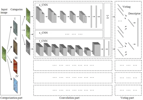
Except the special cases, the correlation between the spatial and temporal properties of the DTs does not exist. Therefore, it is reasonable to introduce the parallel spatial and temporal CNNs called as s-CNN and t-CNN with the finalizing voting of the
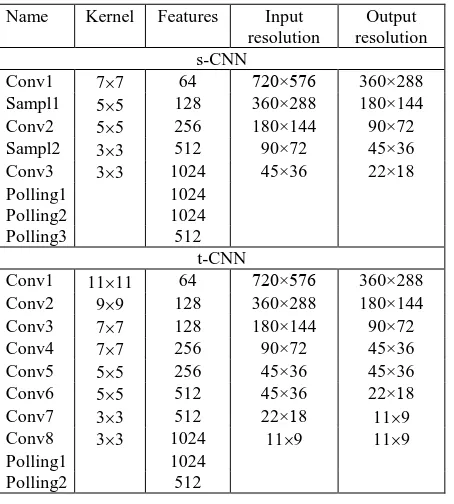
separate concatenated results. The system’s architecture involves three main parts. The first categorization part defines a periodicity activity in a long-term series of the DTs that exceed as minimum in four times a period length of oscillations or it will be clarified that a periodicity is absent. The second convolution part analyses a short-term series and includes two CNNs and one t-CNN for a pair of successive frames. The s-CNNs process two successive frames, while the inputs of the t-CNN obtain a frame difference. The layers of all t-CNNs are trained relative to a category that was determined during a categorization part. For this goal, different spatial and temporal filters are tuned. The output feature results of two s-CNNs are averaged. The third voting part concatenates the spatial and temporal features in order to define a class of the DT. The detailed block-chart of the proposed architecture is depicted in Figure 1. The specifications of two s-CNNs and one t-CNN for category I of the DTs are situated in Table 1. Consider the implementation of the learning and test processes in the DT recognition system in Sections 4.1 and 4.2, respectively.
4.1 Overview of Learning Process
Suppose that two successive training frames of size m n pixels are divided into k k patches, where k is an odd number. In
Figure 1. The detailed block-chart of the proposed architecture
Name Kernel Features Input
Table 1. Specification of the proposed architecture
each convolutional layer, one of the filters is applied to each patch. The s-layer provides an estimation of the obtained intermediate results using a sigmoid function. During a learning stage, only the high quality frames are processed with the goal to tune optimally the parameters of each filter. In current architecture, the mean filter, the median filter, and the Laplacian filter were applied in the s-CNN and four spatiotemporal measures (equations 3-6) were implemented in the t-CNN for four DTs categories. Also the optical flow provides the information about the local and global motion vectors. After the last layer, the residuary patches ought to be binarized and represented as the separate histograms. The goal of the pooling layers is to aggregate the separate histograms, improve their representation, and create the output histogram for a voting part. Note that the output histograms from two s-CNNs are averaged. Each final histogram is associated with the labelled class of the DTs.
4.2 Overview of Test Process
The well-trained CNNs do not need in the architecture changes during a test process. The input frames are categorized according to the movement and main spatial features. The histograms are improved and concatenated in a voting part of a system. For recognition, the Kullback-Leibler distance among the others, such as Chi-square distance, histogram intersection distance, and G-statistics, was used as a recommended frequently method for the histograms’ comparison. Also the Kullback-Leibler distance called as a divergence provided the best results in our previous researches regarding the dynamic transparent textures (Favorskaya et al., 2015).
The Kullback-Leibler divergence is adapted for measuring distances between histograms in order to analyze the probability of occurrence of code numbers for compared textures. First, the probability of occurrence of the code numbers is accumulated into one histogram per image. Each bin in a histogram represents a code number. Second, the constructed histograms of test images are normalized. Third, the Kullback-Leibler divergence DKL is computed by equation 7:
K = the total number of coded numbers
Note that a multi-scale analysis is only required for the DTs from categories III and IV (man-made objects) due to the natural textures are fractals with a self-organizing structure.
5. EXPERIMENTAL RESULTS
The DynTex database (Peteri et al., 2010) includes 678 video sequences with total duration in 337,100 frames or near four and a half hours. All video sequences have the resolution
720×576 pixels. The selected video sequences were divided into four categories, some of which are represented in Tables 2-5.
Description Snapshot Description Snapshot 6ame100.avi
Table 2. Category I (FN is a frame number)
Description Snapshot Description Snapshot 6ammj00.avi
Table 3. Category II (FN is a frame number)
Description Snapshot Description Snapshot 646a510.avi
FN = 650 Flags
6amg500.avi FN = 250 Flag 1
571e110.avi FN = 250 Curtains 1
648e910.avi FN = 250 Flag 2 644ba10.avi
FN = 525 Curtains 2
649bd10.avi FN = 1150 Flag 3 645a930.avi
FN = 250 Decoration
6483910.avi FN = 1425 Leaves 1 645a540.avi
FN = 250 Spruce branches
6486910.avi FN = 250 Leaves 2
Table 4. Category III (FN is a frame number)
Description Snapshot Description Snapshot 54pe210.avi
FN = 250 Escalator
645c510.avi FN = 1200 Highway 1
64ad910.avi FN = 825 Ants
646c410.avi FN = 500 Swarm of birds 64bae10.avi
FN = 250 CD disk
647c730.avi FN = 50 Highway 2 648ab10.avi
FN = 725 Mill
644c310.avi FN = 600 Fan 649i210.avi
FN = 475 Big round thing
6441510.avi FN = 600 Wheel of a bike
Table 5. Category VI (FN is a frame number)
The moving textured objects in video sequences were detected using the block matching algorithm and optical flow. A half of the obtained data was used in the CNN learning, while the other half was applied during the CNN test. Examples of such fragments in color and gray-scale representations are depicted in Figure 2.
Figure 2. Examples of DTs in color and gray-scale representations
Experiments show that the generalized CNN designed for all types of the DTs has very complicated architecture, when only the separate components of the s-layers and c-layers are worked out. This leads to a necessity of preliminary categorization of the DTs with following construction of the specified 2D filters for each type of the DTs. The s-CNN employs Laplacian, Gaussian, the energy Laws filter (Laws, 1980), and the energy Tamura features (Tamura, 1978). The t-CNN uses the filters, employing the block-matching and optical flow components
with the successive decreasing of resolution. Then the resulting histograms are built and compared by the Kullback-Leibler divergence as a measure of differences. As an example, the histograms for Category I and Category III of the DTs are depicted in Figure 3.
Figure 3. Normalized histograms for Category I (blue) and Category III (yellow) of the represented samplings
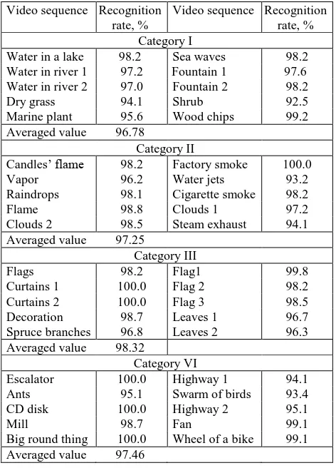
The averaged recognition results for all four Categories are presented in Table 6.
Video sequence Recognition rate, %
Video sequence Recognition rate, % Category I
Water in a lake 98.2 Sea waves 98.2 Water in river 1 97.2 Fountain 1 97.6 Water in river 2 97.0 Fountain 2 98.2
Dry grass 94.1 Shrub 92.5
Marine plant 95.6 Wood chips 99.2 Averaged value 96.78
Category II
Candles’ flame 98.2 Factory smoke 100.0
Vapor 96.2 Water jets 93.2
Raindrops 98.1 Cigarette smoke 98.2
Flame 98.8 Clouds 1 97.2
Clouds 2 98.5 Steam exhaust 94.1
Averaged value 97.25
Category III
Flags 98.2 Flag1 99.8
Curtains 1 100.0 Flag 2 98.2
Curtains 2 100.0 Flag 3 98.5
Decoration 98.7 Leaves 1 96.7
Spruce branches 96.8 Leaves 2 96.3 Averaged value 98.32
Category VI
Escalator 100.0 Highway 1 94.1
Ants 95.1 Swarm of birds 93.4
CD disk 100.0 Highway 2 95.1
Mill 98.7 Fan 99.1
Big round thing 100.0 Wheel of a bike 99.1 Averaged value 97.46
Table 6. Averaged recognition results
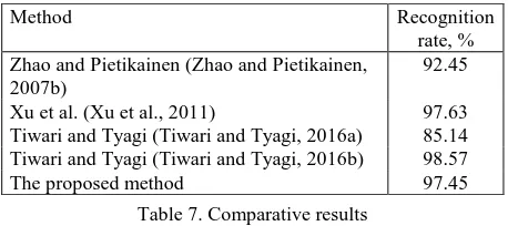
The comparison of the obtained results with the results of other authors was implemented using the DynTex database. The comparative values are placed in Table 7. Note that in most
investigations, the natural DTs are only processed with better results against our averaged results for all DT categories.
Method Recognition
rate, % Zhao and Pietikainen (Zhao and Pietikainen,
2007b)
92.45
Xu et al. (Xu et al., 2011) 97.63
Tiwari and Tyagi (Tiwari and Tyagi, 2016a) 85.14 Tiwari and Tyagi (Tiwari and Tyagi, 2016b) 98.57
The proposed method 97.45
Table 7. Comparative results
The experiments confirm the efficiency of the proposed method for the DTs recognition using the designed CNNs.
6. CONCLUSIONS
The proposed system architecture, including the categorization, convolution and voting parts, provides very promising results in the DT recognition task. The experiments conducted on the sequences from the DynTex database show the best recognition results for the Categories VI and III with the averaged recognition rate 97.46 % and 98.32%, respectively. For the DTs based on man-made opaque rigid objects with stationary or chaotic movement, the errors of temporal features are high for the short-term series that influence on the final result. Also the samples of these categories usually contain a cluttered background. This means that a special attention ought to be paid for the temporal analysis in the further investigations.
ACKNOWLEDGEMENTS
The reported study was funded by the Russian Fund for Basic
Researches according to the research project № 16-07-00121 A.
REFERENCES
Arashloo, S.R., Amirani, M.C., Ardeshir Noroozi, A., 2017. Dynamic texture representation using a deep multi-scale convolutional network. Journal of Visual Communication and Image Representation, 43, pp. 89-97.
Bruna, J., Mallat, S., 2013. Invariant scattering convolution networks. IEEE Transactions on Pattern Analysis and Machine Intelligence, 35(8), pp. 1872-1886.
Chan, A.B., Vasconcelos, N., 2007. Classifying video with kernel dynamic texture. In: The IEEE Conference on Computer Vision and Pattern Recognition, Minneapolis, MN, USA, pp. 1-6.
Chan, T.H., Jia, K., Gao, S., Lu, J., Zeng, Z., Ma, Y., 2015. PCANet: a simple deep learning baseline for image classification? IEEE Transactions on Image Processing, 24(12), pp. 5017-5032.
Chetverikov, D., Peteri, R., 2005 A brief survey of dynamic texture description and recognition. In: The 4th International Conference on Computer Recognition Systems, Rydzyna Castle, Poland, pp. 17–26.
Chetverikov, D., Fazekas, S., 2006. On motion periodicity of dynamic textures. In: The British Machine Vision Conference, Edinburgh, UK, pp. 167-176.
Crivelli, T., Cernuschi-Frias, B., Bouthemy, P., Yao, J., 2013. Motion textures: modeling, classification, and segmentation using mixed-state Markov random fields. SIAM Journal on Imaging Science, 6(4), pp. 2484-2520.
Derpanis, K.G., Wildes, R.P, 2010. Dynamic texture recognition based on distributions of spacetime oriented structure. In: The IEEE Conference on Computer Vision and Pattern Recognition, San Francisco, CA, USA, pp. 1990-1997.
Derpanis, K.G., Wildes, R.P., 2012. Spacetime texture representation and recognition based on a spatiotemporal orientation analysis. IEEE Transactions on Pattern Analysis and Machine Intelligence, 34(6), pp. 1193-1205.
Doretto, G., Chiuso, A., Wu, Y.N., Soatto, S., 2003. Dynamic textures. International Journal on Computer Vision, 51, pp. 91-109.
Doretto, G., Jones, E., Soatto, S., 2004. Spatially homogeneous dynamic textures. In: The European Conference on Computer Vision, Prague, Czech Republic, Vol. 2, pp. 591-602.
Dubois, S., Peteri, R., Menard, M., 2009. A Comparison of Wavelet Based Spatio-temporal Decomposition Methods for Dynamic Texture Recognition. In: The Iberian Conference on Pattern Recognition and Image Analysis, Santiago de Compostela, Spain, pp. 314-321.
Dubois, S., Peteri, R., Menard, M., 2012. Decomposition of Dynamic Textures using Morphological Component Analysis. IEEE Transactions on Circuits and Systems for Video Technology, 22(2), pp. 188-201.
Dubois, S., Peteri, R., Menard, M., 2015. Characterization and recognition of dynamic textures based on 2D+T curvelet transform. Signal, Image and Video Processing, 9(4), pp. 819-830.
Favorskaya, M. (2012) Motion estimation for objects analysis and detection in videos. In: Kountchev, R., Nakamatsu, K. (Eds.) Advances in Reasoning-Based Image Processing Intelligent Systems: Conventional and Intelligent Paradigms. Springer-Verlag, Berlin, Heidelberg, ISRL, Vol. 29, pp. 211-253.
Favorskaya, M., Pyataeva, A., Popov, A., 2015. Verification of smoke detection in video sequences based on spatio-temporal local binary patterns. Procedia Computer Science, 60, pp. 671-680.
Favorskaya, M., Jain, L.C., Proskurin, A., 2016. Unsupervised clustering of natural images in automatic image annotation systems. In: Kountchev, R., Nakamatsu, K. (Eds.) New Approaches in Intelligent Image Analysis: Techniques: Methodologies and Applications. Springer International Publishing, Switzerland, ISRL, Vol. 108, pp. 123-155.
Ghanem, B., Ahuja, N., 2007. Phase based modelling of dynamic textures. In: The IEEE 11th International Conference on Computer Vision, Rio de Janeiro, Brazil, pp. 1-8.
Goodfellow, I., Courville, A., Bengio, Y., 2016. Deep Learning. MIT Press, Cambridge, Massachusetts, London, England.
Haindl, M., Filip, J., 2013. Visual texture: accurate material appearance measurement, representation and modeling. Springer, London, Heidelberg, New York, Dordrecht.
Ji, H., Yang, X., Ling, H., Xu, Y., 2013. Wavelet domain multifractal analysis for static and dynamic texture classification. IEEE Transaction on Image Processing, 22(1), pp. 286-299.
Kanjilal, P.P., Bhattacharya, J., Saha, G., 1999. Robust method for periodicity detection and characterization of irregular cyclical series in terms of embedded periodic components. Physical Review E, 59(4), pp. 4013-4025.
Laws, K.I., 1980. Rapid Texture Identification. In: SPIE 0238, Image Processing for Missle Guardance, San Diego, USA, Vol. 238, pp. 367-380.
Li, J., Chen, L., Cai, Y., 2009. Dynamic texture segmentation using Fourier transform. Modern Applied Science, 3(9), pp. 29-36.
Liu, G., Xia, G.S., Yang, W., Zhang, L., 2014. Texture analysis with shape co-occurrence patterns. In: The 22nd International Conference on Pattern Recognition, Stockholm, Sweden, pp. 1627-1632.
Liu, L., Fieguth, P., Guo, Y., Wang, X., Pietikäinen, M., 2017. Local binary features for texture classification: Taxonomy and experimental study. Pattern Recognition, 62, pp. 135-160.
Oliva, A., Torralba, A., 2001. Modeling the shape of the scene: a holistic representation of the spatial envelope. International Journal on Computer Vision, 42(3), pp. 145-175.
Peteri, R., Chetverikov, D., 2005. Dynamic texture recognition using normal flow and texture regularity. In: The 2nd Iberian Conference on Pattern Recognition and Image Analysis, Estoril, Portugal, pp. 223-230.
Peteri, R., Fazekas, S., Huiskes, M.J., 2010. DynTex: A comprehensive database of dynamic textures. Pattern Recognition Letters, 31(12), pp.1627-1632.
Ravichandran, A., Chaudhry, R., Vidal, R., 2013. Categorizing dynamic textures using a bag of dynamical systems. IEEE Transactions on Pattern Analysis and Machine Intelligence, 35(2), pp. 342-353.
Qi, X., Li,C.G., Zhao,G., Xiaopeng Hong,X., Pietikainen, M., 2016. Dynamic texture and scene classification by transferring deep image features. Neurocomputing, 171(1), pp. 1230-1241.
Saisan, P., Doretto, G., Wu, Y.N., Soatto, S., 2001. Dynamic texture recognition. In: The IEEE Conference on Computer Vision and Pattern Recognition, Kauai, Hawaii, Vol. 2, pp. 58– 63.
Schmidhuber, J., 2015. Deep learning in neural networks: An overview. Neural Networks, 61, pp. 85-117.
Szummer, M., Picard, R.W., 1996. Temporal texture modelling. In: The International Conference on Image Processing, Lausanne, Switzerland, Vol. 3, pp.823-826.
Tamura, H., Mori, S., Yamawaki, T., 1978. Textural features corresponding to visual perception. IEEE Transaction on Systems, Man and Cybernetic, Vol. 8, pp. 400–473.
Tiwari, D., Tyagi, V., 2016a. Dynamic texture recognition: a review. In: Satapathy, S., Mandal, J., Udgata, S., Bhateja, V. (Eds.) Information Systems Design and Intelligent Applications. Springer, New Delhi, Heidelberg, New York, Dordecht, London, AISC, Vol. 434, pp 365–373.
Tiwari, D., Tyagi, V., 2016b. Dynamic texture recognition based on completed volume local binary pattern. Multidimensional Systems and Signal Processing, 27(2), pp. 563-575.
Wildes, R.P., Bergen, J.R., 2000. Qualitative representation. In: The European Conference on Computer Vision, Dublin, Ireland, pp.768-784.
Xu, Y., Quan, Y., Ling, H., Ji, H., 2011. Dynamic texture classification using dynamic fractal analysis. In: The IEEE International Conference on Computer Vision, Barcelona, Spain, pp. 1219-1226.
Xu, Y., Quan, Y., Zhang, Z., Ling, H., Ji, H., 2015. Classifying dynamic textures via spatiotemporal fractal analysis. Pattern Recognition, 48(10), pp. 3239-3248.
Yang, F., Xia, G.S., Liu, G., Zhang, L., Huang, X., 2016. Dynamic texture recognition by aggregating spatial and temporal features via ensemble SVMs. Neurocomputing, 173(Part 3), pp. 1310-1321.
Yang, X., Molchanov, P., Kautz, J., 2016. Multilayer and multimodal fusion of deep neural networks for video classification. In: The ACM Multimedia Conference, Amsterdam, the Netherland, pp. 978-987.
Zhao, G., Pietikainen, M., 2007a. Dynamic texture recognition using local binary patterns with an application to facial expressions. IEEE Transactions on Pattern Analysis and Machine Intelligence, 29(6), pp. 915-928.
Zhao, G., Pietikainen, M., 2007b. Dynamic texture recognition using volume local binary patterns. In: Vidal, R., Heyden, A., Ma, Y. (Eds.) Dynamical Vision. Springer-Verlag, Berlin, Heidelberg, pp. 165-177.
Zhao, G., Ahonen, T., Matas, J., Pietikainen, M., 2012. Rotation-invariant image and video description with local binary pattern features. IEEE Transactions on Image Processing, 21(4), pp. 1465-1477.