Upper and lower bounds for sums of random variables
q
Rob Kaas
a,b,∗, Jan Dhaene
a,b, Marc J. Goovaerts
a,baInstitute of Actuarial Science, University of Amsterdam, Roetersstraat 11, 1018 WB Amsterdam, Netherlands bCRIR, KU Leuven, Belgium
Received March 2000; received in revised form July 2000
Abstract
In this contribution, the upper bounds for sums of dependent random variablesX1+X2+ · · · +Xnderived by using comonotonicity are sharpened for the case when there exists a random variableZsuch that the distribution functions of the
Xi, givenZ = z,are known. By a similar technique, lower bounds are derived. A numerical application for the case of lognormal random variables is given. © 2000 Elsevier Science B.V. All rights reserved.
Keywords:Dependent risks; Comonotonicity; Convex order; Cash-flows; Present values; Stochastic annuities
1. Introduction
In some recent articles, Goovaerts, Denuit, Dhaene, Müller and several others have applied theory originally studied by Fréchet in the previous century to derive upper bounds for sumsS=X1+X2+ · · · +Xnof random variablesX1, X2, . . . , Xn of which the marginal distribution is known, but the joint distribution of the random vectorX1, X2, . . . , Xn is either unspecified or too cumbersome to work with. These upper bounds are actually suprema in the sense of convex order. The concept of convex order is closely related to the notion of stop-loss order which is more familiar in actuarial circles. Both express which of two risks is the more risky one. Assuming that only the marginal distributions of theXi are given (or used), the riskiest instanceSu ofS occurs when the risks X1, X2, . . . , Xnare comonotonous. This means that they are all non-decreasing functions of one uniform (0, 1) random variableU, and since the marginal distribution must be Pr[Xi ≤x]=Fi(x), the comonotonous distribution is that of the vectorF1−1(U ), F2−1(U ), . . . , Fn−1(U ).
In this contribution we assume that the marginal distribution of each random variableX1, X2, . . . , Xnis known. In addition, we assume that there exists some random variableZ, with a known distribution function, such that for anyiand for anyzin the support ofZ, the conditional distribution function ofXi, givenZ=z, is known. We will derive upper and lower bounds in convex order forS=X1+X2+ · · · +Xn, based on these conditional distribution functions. Two extreme situations are possible here. One is thatZ =S, or some one-to-one function of it. Then the convex lower bound forS, which equalsE[S|Z], will just beSitself. The other is thatZis independent of all
X1, X2, . . . , Xn. In this case we actually do not have any extra information at all and the upper bound forSis just the same comonotonous bound as before, while the lower bound reduces to the trivial boundE[S]. But in some
q
Paper presented at the Fourth Conference on Insurance: Mathematics and Economics, Barcelona, 24–26 July 2000.
∗Corresponding author.
E-mail address:[email protected] (R. Kaas).
cases, and the lognormal discount process of Section 5 is a good example, a random variableZcan be found with the property that by conditioning on it we can actually compute a non-trivial lower bound and a sharper upper bound thanSuforS.
In Section 2, we will present a short exposition of the theory we need. Section 3 gives upper bounds, Section 4 improved upper bounds, as well as lower bounds, both applied to the case of lognormal distributions in Section 5. Section 6 gives numerical examples of the performance of these bounds, and Section 7 concludes.
2. Some theory on comonotonous random variables
LetF1, F2, . . . , Fnbe univariate cumulative distribution functions (cdfs in short). Fréchet studied the class of all n-dimensional cdfsFXof random vectorsX≡(X1, X2, . . . , Xn)with given marginal cdfsF1, F2, . . . , Fn, where for any real numberxwe have Pr[Xi ≤x]=Fi(x), i =1,2, . . . , n. In this paper, we will consider the problem of determining stochastic lower and upper bounds for the cdf of the random variableX1+X2+ · · · +Xn, without restricting to independence between the termsXi. We will always assume that the marginals cdfs of theXi are given, and that all cdfs involved have a finite mean.
The stochastic bounds for random variables will be in terms of “convex order”, which is defined as follows:
Definition 1. Consider two random variablesX andY. ThenX is said to precedeY in the convex order sense,
notationX≤cxY, if and only if for all convex real functionsvsuch that the expectations exist, we have
E[v(X)]≤E[v(Y )].
It can be proven, see e.g. Shaked and Shanthikumar (1994), that the condition in this definition is equivalent with the following condition:
E[X]=E[Y], E[X−d]+≤E[Y −d]+ for alld,
whereE[Z]+is a notation forE[max{Z,0}].
Using an integration by parts, the ordering condition between the stop-loss premiumsE[X−d]+andE[Y−d]+ can also be expressed as
Z ∞
d
(1−FX(x))dx≤ Z ∞
d
(1−FY(x))dx for alld.
In caseX ≤cx Y, extreme values are more likely forY than forX. In terms of utility theory,X ≤cx Y entails that lossX is preferred to lossY by all risk averse decision makers, i.e.E[u(−X)]≥E[u(−Y )] for all concave non-decreasing utility functionsu. This means that replacing the (unknown) distribution function of a lossX by the distribution function of a lossY can be considered as an actuarially prudent strategy, e.g. when determining reserves.
From the above relation, we see immediately that
d
dx{E[X−x]+−E[Y −x]+} =FX(x)−FY(x).
Thus, two random variablesXandYwith equal mean are convex ordered if their cdfs cross once. This last condition can be observed to hold in most conceivable examples, but it is easy to construct instances withX≤cxYwhere the cdfs cross more than once.
For any random vectorXwith marginal cdfsF1, F2, . . . , Fnthe following convex order relation holds: X1+X2+ · · · +Xn≤cxSudef=F1−1(U )+F2−1(U )+ · · · +Fn−1(U ),
whereUis a uniform (0, 1) random variable, and where thepth quantile of a random variableXwith cdfFXis, as usual, defined by
FX−1(p)def=inf{x∈R|FX(x)≥p}, p∈[0,1].
Goovaerts et al. (2000) prove this order relation directly, while Müller (1997) derives it as a special case of the concept of supermodular ordering. This relation can be interpreted as follows: the most risky random vector with given marginals (in the sense that the sum of their components is largest in the convex order sense) has thecomonotonous
joint distribution, which means that it has the joint distribution ofF1−1(U ), F2−1(U ), . . . , Fn−1(U ). The components of this random vector are maximally dependent, all components being non-decreasing functions of the same random variable.
The inverse cdf of a sum of comonotonous random variables can easily be computed. Indeed, ifSu=dF1−1(U )+ F2−1(U )+ · · · +Fn−1(U ), where=dmeans equality in distribution, then
FS−1
u (p)=
n X
i=1
Fi−1(p), p∈[0,1].
Recently, the concept of comonotonicity has been considered in many actuarial papers, see e.g. Müller (1997), Wang and Dhaene (1998) and Dhaene et al. (1998). Dependence in portfolios and related stochastic orders are also considered in Dhaene and Goovaerts (1996), Denuit and Lefèvre (1997), Dhaene and Goovaerts (1997), Bäuerle and Müller (1998), Wang and Young (1998), Goovaerts and Redant (1999), Denuit et al. (1999), Dhaene and Denuit (1999) and others.
3. Comonotonous upper bounds for sums of random variables
The usual definition of the inverse of a cdf is the left-continuous functionFX−1(p) =inf{x ∈R|FX(x)≥ p}. But ifFX(x)=pholds for an interval of values forx, any element of it could serve asFX−1(p). In this paper, we introduce a more sophisticated definition which enables us to choose that particular inverse cdf with the property that for a certaind, the relationFX−1(FX(d))=d holds.
Forp∈[0,1], a possible choice for the inverse ofFXinpis any point in the interval
[inf{x ∈R|FX(x)≥p};sup{x ∈R|FX(x)≤p}].
Here we take inf∅ = +∞and sup∅ = −∞. Taking the left-hand side border of this interval to be the value of the inverse cdf atp, we getFX−1(p). Similarly, we defineFX−1•(p)as the right-hand side border of the interval
FX−1•(p)=sup{x ∈R|FX(x)≤p}, p∈[0,1].
Note thatFX−1(0)= −∞andFX−1•(1)= +∞, whileFX−1(p)andFX−1•(p)are finite for allp∈(0,1). For anyα
in [0,1], we define theα-inverse ofFXas follows:
FX−1(α)(p)=αFX−1(p)+(1−α)FX−1•(p), p∈(0,1).
For a comonotonous random vector(X1, X2, . . . , Xn), it follows that for allαin [0,1]
FX−1(α)
1+X2+···+Xn(p)=
n X
i=1 FX−1(α)
The following result was already mentioned in Section 1. We give a new proof for it, based on theα-inverse just introduced, because this method of proof leads to new results that we will need in the sequel of this paper.
Proposition 1. Let U be a uniform(0,1)random variable. For any random vector(X1, X2, . . . , Xn)with marginal
cdfsF1, F2, . . . , Fn,we have
X1+X2+ · · · +Xn≤cxF1−1(U )+F2−1(U )+ · · · +Fn−1(U ).
Proof. LetS andSu be defined byS =X1+X2+ · · · +Xn andSu = F1−1(U )+F2−1(U )+ · · · +Fn−1(U ),
respectively, withU uniform (0, 1). Then obviously E[S] = E[Su]. To prove the stop-loss inequalities needed to establish convex order, consider an arbitrary fixed real numberd, with 0 < FSu(d) < 1. Let α ∈ [0,1] be
On the other hand we find
E[Su−d]+=E[FS−u1(U )−d]+=
As the stop-loss transform is a continuous, non-increasing function of the retentiond, we find that the result above implies
E[S−FS−1•
u (0)]+≤E[Su−F
as well as
stop-loss premium at retention d ofSuis given by
E[Su−d]+=
The expression for the stop-loss premiums of a comonotonous sumSucan also be written in terms of the usual inverse cdfs. Indeed, for any retentiond∈(FS−1•
Summing overi, and taking into account the definition ofα, we find the expression derived in Dhaene et al. (1998), where the random variables are assumed to be non-negative
E[Su−d]+=
From Corollary 1, we can conclude that any stop-loss premium of a sum of comonotonous random variables can be written as the sum of stop-loss premiums for the individual random variables involved. Corollary 1 provides an algorithm for directly computing stop-loss premiums of sums of comonotonous random variables, without having to compute the entire cdf of the sum itself. Indeed, in order to compute the stop-loss premium with retentiond, we only need to knowFSu(x)forxequal tod. The cdf atxfollows from can verify thatFSuis also continuous onRand strictly increasing on(F−
1•
In this case, we also find
E[Su−d]+=
4. Improved bounds for sums of random variables
4.1. Upper bounds
As(F1−1(U ), F2−1(U ), . . . , Fn−1(U ))is a random vector with marginals F1, . . . , Fn, the upper bound Su = F1−1(U )+F2−1(U )+ · · · +Fn−1(U )is the best that can be derived under the conditions stated in Proposition 1; it is a supremum in terms of convex order. Let us now assume that we have complete (or partial) information, more than just the marginal distributions, concerning the dependence structure of the random vector(X1, X2, . . . , Xn), but that exact computation of the cdf of the sumS=X1+X2+ · · · +Xnis not feasible. In this case, we will show that it is possible to derive improved upper bounds forS, and also non-trivial lower bounds, based on the information we have on the dependence structure. This is accomplished by conditioning on a random variableZwhich is assumed to be some function of the random vectorX. We will assume that we know the distribution ofZ, and also the conditional cdfs, givenZ=z, of the random variablesXi. A suitable example is to useZ=PlogXiwhen theXi are lognormal. In the following proposition, we introduce the notationFX−1
i|Z(U )for the random variablefi(U, Z),
where the functionfiis defined byfi(u, z)=FX−i1|Z=z(u).
Proposition 2. Let U be uniform(0,1),and consider a random variable Z which is independent of U. Then we
have
Proof. From Proposition 1, we get for any convex functionv,
E[v(X1+ · · · +Xn)]=
from which the stated result follows directly.
Note that the random vector(FX−1
In view of Proposition 1 this implies
FX−1
The left-hand side of this relation isSu′; the right-hand side isSu. In order to obtain the distribution function ofSu′, observe that given the eventZ=z, this random variable is a sum of comonotonous random variables. Hence
The cdf ofSu′ then follows from
FS′
u(x)=
Z ∞
−∞ FS′
u|Z=z(x)dFZ(z).
Application of Proposition 2 to lognormal marginalsXiis considered in Section 5, but see also the simple examples withn=2 at the end of this section. Note that ifZis independent of allX1, X2, . . . , Xn, upper boundSu′ reduces toSu.
4.2. Lower bounds
LetXbe a random vector with marginalsF1, F2, . . . , Fn, and assume that we want to find a lower boundSl, in the sense of convex order, forS =X1+X2+ · · · +Xn. We can obtain such a bound by conditioning on some random variableZ, again assumed to be a function of the random vectorX.
Proposition 3. For any random vectorXand random variable Z, we have
Sldef=E[X1|Z]+E[X2|Z]+ · · · +E[Xn|Z]≤cxX1+X2+ · · · +Xn.
Proof. By Jensen’s inequality, we find that for any convex functionv, the following inequality holds:
E[v(X1+X2+ · · · +Xn)]=EZE[v(X1+X2+ · · · +Xn)|Z]≥EZ[v(E[X1+X2+ · · · +Xn|Z])] =EZ[v(E[X1|Z]+ · · · +E[Xn|Z])].
This proves the stated result.
Note that ifZandSare mutually independent, Proposition 3 leads to the trivial lower boundE[S]≤cxS. On the other hand, ifZandShave a one-to-one relation, the lower bound in Proposition 3 coincides withS. Note further that
E[E[Xi|Z]]=E[Xi] always holds, but Var[E[Xi|Z]]<Var[Xi] unlessE[Var[Xi|Z]]=0 which means thatXi, givenZ=z, is a constant for eachz. This implies that the random vector(E[X1|Z], E[X2|Z], . . . , E[Xn|Z])will in general not haveF1, F2, . . . , Fn as its marginal distribution functions. But if the conditioning random variable Zhas the property that all random variablesE[Xi|Z] are non-increasing functions ofZ(or all are non-decreasing functions ofZ), the lower bound in Proposition 3 has the form of a sum ofncomonotonous random variables. The cdf of this sum is then obtained by the results of Section 2. An application of Proposition 3 in the case of lognormal marginalsXiis considered in Section 5.
WithS =X1+X2+ · · · +Xn, the lower boundSl in Proposition 3 can be written asE[S|Z]. To judge the quality of this stochastic bound, we might look at its variance. To maximize it, the mean value of Var[S|Z = z] should be minimized. Thus, for the best lower bound,ZandSshould be as alike as possible.
Let us further assume that the random variableZis such that allE[Xi|Z] are non-increasing continuous functions ofZ. The quantiles of the random variableE[S|Z] then follow from
FE−[1S|Z](p)= n X
i=1 FE−[1X
i|Z](p)=
n X
i=1
E[Xi|Z=FZ−1(1−p)], p∈(0,1).
In order to derive the above result, we used the fact that for a non-increasing continuous functionf, we have
Ff (S)−1 (p)=f (FS−1(1−p)), p∈(0,1).
Similarly, for a non-decreasing continuous functionf, we have
If we now in addition assume that the cdfs of the random variables E[Xi|Z] are strictly increasing and
con-The stop-loss premiums ofE[S|Z] can be computed as follows:
E[E[S|Z]−d]+=
The technique for deriving lower bounds as explained in this section is also considered (for some special cases) in Vyncke et al. (2000). The idea of this technique stems from mathematical physics, and was applied by Rogers and Shi (1995) to derive approximate values for the value of Asian options.
4.3. Some simple examples
LetX, Y be independentN (0,1)random variables, and consider random variables of the typeZ=X+aYfor some reala. We want to derive stochastic bounds forS=X+Y. The conditional distribution ofX, givenZ=z, tonous. For the lower and upper bounds derived above we get
Su′ = 1+a
1+a2Z+
1+ |a| (1+a2)1/2Φ
−1(U ) ∼N
0,(1+a) 2
+(1+ |a|)2
1+a2
,
Su=d2X∼N (0,4).
For some special choices ofa, we get the following distributions for the lower and upper boundsSl andSu′:
a=0 : N (0,1)≤cxS≤cxN (0,2),
a=1 : N (0,2)≤cxS≤cxN (0,4),
a= −1 : N (0,0)≤cxS≤cxN (0,2),
|a| → ∞: N (0,1)≤cxS≤cxN (0,2).
Note that the actual distribution ofSisN (0,2), so the best convex lower bound(a=1)and the best upper bound
(a ≤ 0 ora → ∞)coincide withS. Of course taking |a| → ∞gives the same results as takingZ = Y. The variance ofSl can be seen to have a maximum ata= +1, a minimum ata = −1. On the other hand, Var[S′u] also has a maximum ata =1, and minima ata ≤ 0 anda → ∞. So the best lower bound in this case is attained for
Z=S, the worst forZandSindependent. The best improved upper bound is found by takingZ=X,Z=Y, or anya <0, including the casea= −1 withZandSindependent; the worst, however, by takingZ =S.
To compare the variance of the stochastic upper bound Su′ with the variance of S boils down to comparing cov(FX−|1Z(U ), FY−|1Z(U ))with cov(X, Y ). It is clear that, in general, the optimal choice for the conditioning random variableZwill depend on the correlation ofXandY. If this correlation equals 1, anyZresults inS=dS′u=dS. In our case whereXandY are mutually independent, the optimal choice proves to be takingZ≡XorZ≡Y, thus ensuring thatSandSu′ coincide.
As a second example, consider a simple special case of the theory dealt in the next section. We present it here for the reader’s convenience, just as an illustration. TakeY1andY2be independentN (0,1)random variables. Look at
the sum ofX1 =eY1 ∼lognormal(0,1), andX2=eY1+Y2 ∼lognormal(0,2). TakeZ =Y1+Y2. For the lower
boundSl, note thatE[X2|Z]=eZ, whileY1|Y1+Y2=z∼N (12z,12), hence E[eY1
|Y1+Y2=z]=m(1;12z,12),
wherem(t;µ, σ2)=exp(µt+21σ2t2)is theN (µ, σ2)moment generating function. This leads to
E[eY1
|Z]=exp(12Z+14).
So the lower bound is
Sl =E[X1+X2|Z]=exp(12Z+14)+eZ.
Upper boundSu has(X1, X2)=d (eW,e √
2W)forW
∼N (0,1). The improved upper boundSu′ has as a second term again eZ, and as first term exp(12Z+21√2W ), withZandWmutually independent. All terms occurring in the bounds given above are lognormal random variables, so the variances of the bounds are easy to compute. Note that to compare variances is meaningful when comparing stop-loss premiums of stop-loss ordered random variables, see, e.g., Kaas et al. (1994, p. 68). The following relation, which can be proven using partial integration, links variances and stop-loss premiums:
1
2Var[X]= Z ∞
−∞{
E[X−t]+−(E[X]−t )+}dt,
from which we deduce that ifX≤cxY, thusE[Y −t]+≥E[X−t]+for allt, then
1
2{Var[Y]−Var[X]} = Z ∞
−∞{
Thus, half the variance difference between two convex ordered random variables equals the integrated difference of their stop-loss premiums. This implies that ifX ≤cx Y and in addition Var[X]=Var[Y], thenX andY must necessarily be equal in distribution. Moreover, the ratio of the variances is roughly equal to the ratio of the stop-loss premiums, minus their minimal possible value for random variables with the same mean. We have, as the reader may verify,
E[S]2=e1+2e5/2+e4, E[Sl2]=e3/2+2e5/2+e4, E[S2]=E[Su′2]=e2+2e5/2+e4, E[Su2]=e2+2e3/2+
√ 2
+e4.
Hence
Var[E[S]]=0, Var[Sl]=1.763, Var[S]=Var[Su′]=4.671, Var[Su]=17.174.
So an improved stochastic lower boundSl forS is obtained by conditioning onY1+Y2, and the improved upper
boundSu′ for this case proves to be very good indeed, having in fact the same distribution asS.
5. Present values — lognormal discount process
5.1. General result
Consider a series of deterministic paymentsα1, α2, . . . , αn, of arbitrary sign, that are due at times 1,2, . . . , n, respectively. The present value of this series of payments equals
S= n X
i=1
αiexp(−(Y1+Y2+ · · · +Yi)).
Assume that(Y1, Y2, . . . , Yn)has a multivariate normal distribution. We introduce the random variablesXi and Y (i)defined by
Y (i)=Y1+Y2+ · · · +Yi; Xi =αie−Y (i). thenS =X1+X2+ · · · +Xn.
For some given choice of theβi, consider a conditioning random variableZdefined as follows:
Z= n X
i=1 βiYi,
For a multivariate normal distribution, every linear function of its components has a univariate normal distribution, soZis normally distributed. Also,(Y (i), Z)has a bivariate normal distribution. Conditionally givenZ =z,Y (i)
has a univariate normal distribution with mean and variance given by
E[Y (i)|Z=z]=E[Y (i)]+ρi σY (i)
σZ
(z−E[Z]),
and
Var[Y (i)|Z =z]=σY (i)2 (1−ρi2),
Proposition 4. LetS, Sl, Su′ andSube defined as follows:
where U and V are mutually independent uniform(0,1)random variables, andΦis the cdf of theN (0,1)distribution. Then we have
3. The stochastic inequalitySu′ ≤cxSufollows from Proposition 1.
In order to compare the cdf ofS=Pn
i=1αiexp(−(Y1+Y2+ · · · +Yi))with the cdfs ofSl, Su′ andSu, especially their variances, we need the correlations of the different random variables involved. We find the following results for the lognormal discount process considered in this section:
From these correlations, we can for instance deduce that if all paymentsαi are positive and corr[Y (i), Y (j )]=1 for alliandj, thenS=dSu. In practice, the discount factors will not be perfectly correlated. But for any realistic discount process, corr[Y (i), Y (j )]=corr[Y1+ · · · +Yi, Y1+ · · · +Yj] will be close to 1 provided thatiandj are close to each other. This gives an indication that the cdf ofSumight perform well as approximation for the cdf ofSfor such processes. This is indeed the case in the numerical illustrations in Goovaerts et al. (2000). A similar reasoning leads to the conclusion that the cdf ofSu will not perform well as a convex upper bound for the cdf of Sif the paymentsαi have mixed signs. This phenomenon will indeed be observed in the numerical illustrations in Section 6.
It remains to derive expressions for the cdfs ofSl, Su′ andSu.
5.2. The cdf and the stop-loss premiums ofSu
The quantiles ofSufollow from Goovaerts et al. (2000)
FS−1
u (p)=
n X
i=1
αiexp(−E[Y (i)]+sign(αi)σY (i)Φ−1(p)), p∈(0,1).
Also,FSu(x)follows implicitly from solving
n X
i=1
αiexp(−E[Y (i)]+sign(αi)σY (i)Φ−1(FSu(x)))=x.
It is straightforward to derive expressions for the stop-loss premiums in this case
E[Su−d]+= n X
i=1
|αi|e−E[Y (i)]E[sign(αi)(Zi−exp(sign(αi)σY (i)Φ−1(FSu(d))))]+,
where theZiare lognormal(0, σY (i)2 ) random variables.
In order to derive an explicit expression for the stop-loss premiumsE[Su−d]+, we first mention the following result, which can easily be proven, e.g. by using(d/dt )E[X−t]+=FX(t )−1.
Proposition 5. If Y is lognormal(µ, σ2),then for anyd >0we have
E[Y −d]+=exp(µ+21σ2)Φ(d1)−dΦ(d2), E[Y −d]−=exp(µ+12σ2)Φ(−d1)−dΦ(−d2),
whered1andd2are determined by
d1=
µ+σ2−ln(d)
σ , d2=d1−σ.
Atd ≤ 0,the stop-loss premiums are trivially equal toE[Y]−d. The following expression results for the stop-loss premiums atd >0:
E[Su−d]+= n X
i=1
αie−E[Y (i)]{exp(21σY (i)2 )Φ(sign(αi)di,1)
−exp(sign(αi)σY (i)Φ−1(FSu(d)))Φ(sign(αi)di,2)}
withdi,1anddi,2given by
di,1=σY (i)−sign(αi)Φ−1(FSu(d)), di,2= −sign(αi)Φ−
Using the implicit definition forFSu(d)leads to the following expression for the stop-loss premiums:
5.3. The cdf and the stop-loss premiums ofSl
In general,Slwill not be a sum ofncomonotonous random variables. But in the remainder of this subsection, we assume that allαi ≥0 and allρi =cov[Y (i), Z]/σY (i)σZ ≥0. These conditions ensure thatSlis the sum ofn comonotonous random variables.
Taking into account thatZ=Pn
i=1βiYi is normally distributed, we find that
After some straightforward computations, one finds that an explicit expression for the stop-loss premiums is given by
E[Sl−d]+=
u|U=uis a sum ofncomonotonous random variables, we have
6. Numerical illustration
In this section, we will numerically illustrate the bounds we derived forS=Pn
i=1αiexp(−(Y1+Y2+ · · · +Yi)). We will taken=20. In order to be able to compare the distribution functions of the stochastic boundsSl, S′uandSu with the distribution function ofS, we will completely specify the multivariate distribution function of the random vector(Y1, Y2, . . . , Y20). In particular, we will assume that the random variablesYi are i.i.d. andN (µ, σ2). This will enable us to simulate the cdfs in case there is no way to compute them analytically. The conditioning random variableZis defined as before
Z=
In our numerical illustrations, we will choose the parameters of the normal distribution involved as follows:
µ=0.07, σ =0.1.
We will compute the lower bound and the upper bound for the following choice of the parametersβi:
βi = 20
X
j=i
αje−j µ, i=1, . . . ,20.
By this choice, the lower bound will perform well in these cases. This is due to the fact that this choice makesZa linear transformation of a first-order approximation toS. This can be seen from the following computation, which depends onσ, and henceYi−µ, being “small”:
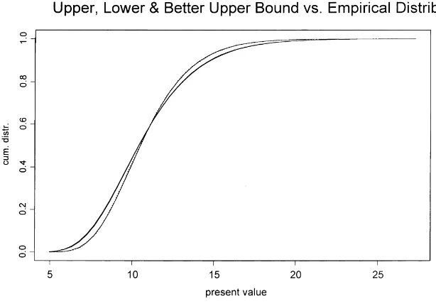
whereCis the appropriate constant. By the remarks in Section 4,Slwill then be “close” toS. Fig. 1 shows the cdfs ofS, Sl, Su′ andSufor the following payments:
αk =1, k=1, . . . ,20.
SinceSl ≤cxS≤cxSu′ ≤cxSu, and the same ordering holds for the tails of their distribution functions which can be observed to cross only once, we can easily identify the cdfs. We see that the cdf ofSlis very close to the distribution ofS, which was expected because of the choice ofZ. Note that in this caseSl is a sum of comonotonous random variables, so its quantiles can be computed easily. The cdf ofSu also performs rather well, as was observed in Goovaerts et al. (2000). We find that the improved upper boundSu′ is very close to the comonotonous upper bound
Su. This is due to the fact that cov(FX−i1|Z(U ), F
−1
Fig. 1. Payments: 20×1;Zis such that the lower bound is optimized.
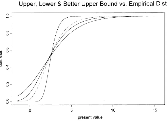
Fig. 2 shows the cdfs ofS, Sl, Su′ andSufor the following payments:
αk =
−1, k=1, . . . ,5,
1, k=6, . . . ,20.
Note that the cdf of the lower boundSlcannot be computed exactly in this case; it is obtained by simulation. In this case, we see that the lower boundSl still performs very well. The comonotonous upper boundSu performs very
Fig. 3. Payments: 5×(−1),15×1;Zis such that it is an approximation to the discounted total of the negative payments.
badly in this case, as was to be expected from the observations in Section 5.1. The improved upper bound performs better.
In Fig. 3, we consider the same series of payments as in Fig. 2. We consider the cdf of the improved upper bound for a different choice of the conditioning random variableZ. We chooseZsuch that it is an approximation to the discounted total of the five negative payments:
βi = P5
j=iαje−j µ, i=1, . . . ,5, 0, i=6, . . . ,20.
The (simulated) cdf ofSis the dotted line. Note that the upper boundSu′ is much improved, the lower bound is worse.
7. Conclusions and related research
when one wants to determine fair values and supervisory values. But note that Pr[S ≤ x] cannot be guaranteed to be between Pr[Sl ≤x] and Pr[Su′ ≤ x]. It has been argued before, see e.g. Kaas (1994), that actuaries should not be focused on probabilities and quantiles, but rather on stop-loss premiums, since it is not the probability of exceeding a thresholddthat matters, but the amount by which this happens, of which the expected value is just the stop-loss premium atd. And for stop-loss premiums, the propertyE[Sl−d]+ ≤E[S−d]+≤E[Su′ −d]+does hold.
It should be noted that the upper boundSu′ is no longer a supremum (in the sense of convex order) over the set of all random vectors with fixed marginals, and that the lower boundSlis not a sum of terms with the proper marginal distributions. This follows from the fact that the bounds that we derived take into account the dependency structure of the random vector under consideration.
It should also be noted that our results actually do not require the complete dependency structure, but only the distribution ofZ and the conditional distributions ofXi givenZ =z. In Section 6 we chose an example where the distribution of the random vector was completely known, in order to be able to compare the bounds with the (simulated) exact cdf.
A topic for future research is the determination of the optimal conditioning random variableZfor the improved upper boundSu′, in the spirit of the remarks made at the end of Section 4.3. Another item for future research is the extension of the results of this paper to the case where also the cash flows are stochastic, hence to find improved upper bounds and lower bounds forS =X1Y1+X2Y2+ · · · +XnYn. Another idea that we intend to pursue is conditioning on more than one random variableZ.
Acknowledgements
The authors would like to thank Etienne De Vylder for helpful and insightful comments on an earlier version of this paper, and David Vyncke for providing the numerical illustrations of Section 6. Marc Goovaerts and Jan Dhaene acknowledge the financial support of the Onderzoeksfonds K.U. Leuven (grant OT/97/6) and of FWO (grant “Actuarial ordering of dependent risks”).
References
Bäuerle, N., Müller, A., 1998. Modeling and comparing dependencies in multivariate risk portfolios. ASTIN Bulletin 28, 59–76.
Brockett, P., Garven, J., 1998. A reexamination of the relationship between preferences and moment orderings by rational risk averse investors. Geneva Papers on Risk and Insurance Theory 23, 127–137.
Denuit, M., Lefèvre, C., 1997. Stochastic product orderings, with applications in actuarial sciences. Bulletin Français d’Actuariat 1, 61–82. Denuit, M., De Vylder, F., Lefèvre, C., 1999. Extrema with respect tos-convex orderings in moment spaces: a general solution. Insurance:
Mathematics and Economics 24, 201–217.
Dhaene, J., Denuit, M., 1999. The safest dependency structure among risks. Insurance: Mathematics and Economics 25, 11–21. Dhaene, J., Goovaerts, M., 1996. Dependency of risks and stop-loss order. ASTIN Bulletin 26, 201–212.
Dhaene, J., Goovaerts, M.J., 1997. On the dependency of risks in the individual life model. Insurance: Mathematics and Economics 19, 243–253. Dhaene, J., Wang, S., Young, V., Goovaerts, M.J., 1998. Comonotonicity and maximal stop-loss premiums. Research Report 9730. DTEW, KU
Leuven, p. 13, submitted for publication.
Goovaerts, M.J., Redant, R., 1999. On the distribution of IBNR reserves. Insurance: Mathematics and Economics 25, 1–9.
Goovaerts, M.J., Dhaene, J., De Schepper, A., 2000. Stochastic upper bounds for present value functions. Journal of Risk and Insurance Theory 67.1, 1–14.
Kaas, R., 1994. How to (and how not to) compute stop-loss premiums in practice. Insurance: Mathematics and Economics 13, 241–254. Kaas, R., Van Heerwaarden, A.E., Goovaerts, M.J., 1994. Ordering of actuarial risks. Institute for Actuarial Science and Econometrics, University
of Amsterdam, Amsterdam, p. 144.
Müller, A., 1997. Stop-loss order for portfolios of dependent risks. Insurance: Mathematics and Economics 21, 219–223. Rogers, L.C.G., Shi, Z., 1995. The value of an Asian option. Journal of Applied Probability 32, 1077–1088.
Shaked, M., Shanthikumar, J.G., 1994. Stochastic Orders and Their Applications. Academic Press, New York, p. 545.
Vyncke, D., Goovaerts, M.J., Dhaene, J., 2000. Convex upper and lower bounds for present value functions, Research Report 0025, Dept. of Applied Economics, KU Leuven, Belgium.
Wang, S., Dhaene, J., 1998. Comonotonicity, correlation order and stop-loss premiums. Insurance: Mathematics and Economics 22 (3), 235–243. Wang, S., Young, V., 1998. Ordering risks: expected utility versus Yaari’s dual theory of choice under risk. Insurance: Mathematics and