Monodromy of a Class of Logarithmic Connections
on an Elliptic Curve
Francois-Xavier MACHU
Math´ematiques - bˆat. M2, Universit´e Lille 1, F-59655 Villeneuve d’Ascq Cedex, France
E-mail: [email protected]
Received March 22, 2007, in final form August 06, 2007; Published online August 16, 2007 Original article is available athttp://www.emis.de/journals/SIGMA/2007/082/
Abstract. The logarithmic connections studied in the paper are direct images of regular connections on line bundles over genus-2 double covers of the elliptic curve. We give an explicit parametrization of all such connections, determine their monodromy, differential Galois group and the underlying rank-2 vector bundle. The latter is described in terms of elementary transforms. The question of its (semi)-stability is addressed.
Key words: elliptic curve; ramified covering; logarithmic connection; bielliptic curve; genus-2 curve; monodromy; Riemann–Hilbert problem; differential Galois group; elementary trans-formation; stable bundle; vector bundle
2000 Mathematics Subject Classification: 14D21; 14H52; 14H60; 32S40
1
Introduction
The Riemann–Hilbert correspondence relates the integrable logarithmic (or Fuchsian) connec-tions over an algebraic varietyX to the representations of the fundamental groupπ1(X\ {D}), where Ddenotes the divisor of poles of a connection. Deligne [3] proved its bijectivity, on con-dition that D is a fixed normal crossing divisor and the data on both sides are taken modulo appropriate equivalence relations. Nevertheless, Deligne’s solution is not effective in the sense that it does not imply any formulas to compute the Riemann–Hilbert correspondence. Therefore, it is important to have on hand a stock of examples that can be solved explicitly.
The authors of [13, 5] constructed logarithmic connections of rank n over P1 with quasi-permutation monodromy in terms of theta functions on a ramified cover of P1 of degree n. Korotkin in [12] considers a class of generalized connections, called connections with constant twists, and constructs such twisted connections of rank 2 with logarithmic singularities on an elliptic curve E via theta functions on a double cover C of E.
In the present paper, we obtain genuine (non-twisted) rank-2 connections onEfrom its double coverC by a different method, similar to the method applied in [15] to the double covers ofP1. We consider a genus-2 cover f :C→E of degree 2 with two branch pointsp+,p− and a regular
connection ∇L on a line bundle L over C. Then the sheaf-theoretic direct image E = f∗(L) is a rank-2 vector bundle carrying the connection ∇E := f∗(∇L) with logarithmic poles at p+ and p−. We explicitly parameterize all such connections and their monodromy representations
ρ : π1(E \ {p−, p+})→GL(2,C). We also investigate the abstract group-theoretic structure of the obtained monodromy groups as well as their Zariski closures in GL(2,C), which are the differential Galois groups of the connections ∇E.
We also illustrate the following Bolibruch–Esnault–Viehweg Theorem [7]: any irreducible logarithmic connection over a curve can be converted by a sequence of Gabber’s transforms into a logarithmic connection with same singularities and same monodromy on a semistable vector bundle of degree 0. Bolibruch has established this result in the genus-0 case, in which “semistable of degree 0” means just “trivial” [1].
We explicitly indicate a Gabber’s transform of the above direct image connection (E,∇E) which satisfies the conclusion of the Bolibruch–Esnault–Viehweg Theorem. The importance of results of this type is that they allow us to consider maps from the moduli space of connections to the moduli spaces of vector bundles, for only semistable bundles have a consistent moduli theory. Another useful feature of the elementary transforms is that they permit to change arbitrarily the degree, and this enriches our knowledge of the moduli space of connections providing maps to moduli spaces of vector bundles of different degrees, which may be quite different and even have different dimensions (see Remark 2).
All the relevant algebro-geometric tools are introduced in a way accessible to a non-specialist. One of them is the usage of ruled surfaces in finding line subbundles of rank-2 vector bundles. This is classical, see [14] and references therein. Another one is the reconstruction of a vector bundle from the singularities of a given connection on it. Though it is known as a theoreti-cal method [6,7], it has not been used for a practical calculation of vector bundles underlying a given meromorphic connection over a Riemann surface different from the sphere. For the Riemann sphere, any vector bundle is the direct sum of the line bundles O(ki), and Bolibruch
developed the method of valuations (see [1]) serving to calculate the integers ki for the
un-derlying vector bundles of connections. He exploited extensively this method, in particular in his construction of counter-examples to the Riemann–Hilbert problem for reducible representa-tions.
Genus-2 double covers of elliptic curves is a classical subject, originating in the work of Legendre and Jacobi [9]. We provide several descriptions of them, based on a more recent work [4]. We determine the locus of their periods (Corollary 1), a result which we could not find elsewhere in the literature and which we need for finding the image of the Riemann–Hilbert correspondence in Proposition 5.
Now we will briefly survey the contents of the paper by sections. In Section2, we describe the genus-2 covers of elliptic curves of degree 2 and determine their periods. In Section 3, we investigate rank-1 connections on C and discuss the dependence of the Riemann–Hilbert cor-respondence for these connections on the parameters of the problem: the period of C and the underlying line bundle L. In Section 4, we compute, separately for the cases L = OC and
L 6= OC, the matrix of the direct image connection ∇E on E = f∗L. For L = OC, we also provide two different forms for a scalar ODE of order 2 equivalent to the 2×2 matrix equa-tion ∇Eϕ = 0. In Section 5, we determine the fundamental matrices and the monodromy of connections ∇E and discuss their isomonodromy deformations. Section 6 introduces the
ele-mentary transforms of rank-2 vector bundles, relates them to birational maps between ruled surfaces and states a criterion for (semi)-stability of a rank-2 vector bundle. In Section 7, we apply the material of Section 6 to describe E as a result of a series of elementary trans-forms starting from E0 =f∗OC and prove its stability or unstability depending on the value of parameters. We also describe Gabber’s elementary transform which illustrates the Bolibruch– Esnault–Viehweg Theorem and comment briefly on the twisted connections of [12]. In Sec-tion 8, we give a description of the structure of the monodromy and differential Galois groups for∇E.
2
Genus-2 covers of an elliptic curve
In this section, we will describe the degree-2 covers of elliptic curves which are curves of genus 2.
Definition 1. Let π :C→E be a degree-2 map of curves. If E is elliptic, then we say that C
is bielliptic and thatE is a degree-2 elliptic subcover ofC.
Legendre and Jacobi [9] observed that any genus-2 bielliptic curve has an equation of the form
y2=c0x6+c1x4+c2x2+c3 (ci ∈C) (1)
in appropriate affine coordinates (x, y). It immediately follows that any bielliptic curveC has two elliptic subcovers πi :C→Ei,
E1 : y2=c0x13+c1x21+c2x1+c3, π1 : (x, y)7→(x1 =x2, y), and
E2 : y22=c3x23+c2x22+c1x2+c0, π2 : (x, y)7→(x2 = 1/x2, y2 =y/x3). (2)
This description of bielliptic curves, though very simple, depends on an excessive number of parameters. To eliminate unnecessary parameters, we will represent Ei in the form
Ei :yi2=xi(xi−1)(xi−ti) (ti ∈C\ {0, 1}, t16=t2). (3)
Remark that any pair of elliptic curves (E1, E2) admits such a representation even if E1≃E2. We will describe the reconstruction ofC starting from (E1, E2) following [4]. This procedure will allow us to determine the periods of bielliptic curves C in terms of the periods of their elliptic subcovers E1,E2.
Let ϕi : Ei→P1 be the double cover map (xi, yi) 7→ xi (i = 1,2). Recall that the fibered
product E1×P1 E2 is the set of pairs (P1, P2)∈E1×E2 such that ϕ1(P1) =ϕ2(P2). It can be
given by two equations with respect to three affine coordinates (x, y1, y2):
C :=E1×P1 E2 :
(
y2
1 =x(x−1)(x−t1),
y22 =x(x−1)(x−t2).
It is easily verified that C has nodes over the common branch points 0, 1, ∞ of ϕi and is
nonsingular elsewhere. For example, locally at x = 0, we can choose yi as a local parameter
on Ei, so that x has a zero of order two onEi; equivalently, we can write x = fi(yi)y2i where
fi is holomorphic and fi(0) 6= 0. Then eliminating x, we obtain that C is given locally by
a single equation f1(y1)y12 = f2(y2)y22. This is the union of two smooth transversal branches p
f1(y1)y1=± p
f2(y2)y2.
Associated toC is its normalization (or desingularization)C obtained by separating the two branches at each singular point. Thus C has two points over x= 0, whilst the only point of C
overx= 0 is the node, which we will denote by the same symbol 0. We will also denote by 0+, 0−
the two points ofC over 0. Any of the functionsy1,y2 is a local parameter at 0±. In a similar
way, we introduce the points 1,∞ ∈C and 1±,∞±∈C.
Proposition 1. Given a genus-2 bielliptic curve C with its two elliptic subcovers πi :C→Ei, one can choose affine coordinates for Ei in such a way that Ei are given by the equations (3),
C is the normalization of the nodal curve C := E1 ×P1 E2, and πi = pri◦ν, where ν :C→C
denotes the normalization map and pri the projection onto thei-th factor.
It is interesting to know, how the descriptions given by (1) and Proposition1 are related to each other. The answer is given by the following proposition.
Proposition 2. Under the assumptions and in the notation of Proposition1, apply the following changes of coordinates in the equations of the curves Ei:
(xi, yi)→(˜xi,y˜i), x˜i=
Further, C can be given by the equation
η2 =
Proof . We have the following commutative diagram of double cover maps
C
The locus of bielliptic curves in the moduli space of all the genus-2 curves is 2-dimensional, hence is a hypersurface. In [16], an explicit equation of this hypersurface is given in terms of the Igusa invariants of the genus-2 curves. We will give a description of the same locus in terms of periods. We start by recalling necessary definitions.
Leta1,a2,b1,b2 be a symplectic basis ofH1(C,Z) for a genus-2 curveC, and ω1,ω2 a basis of the space Γ(C,Ω1C) of holomorphic 1-forms on C.
Definition 2. Let us introduce the 2×2-matrices A = (R
aiωj) and B = ( R
biωj). Their
+
0_
0+
1_
1+
8
+
8 _ t
1_
t
2+
t
2_
a
1
a
2
b
1
b
2
t
1+ ++
_ _
+ _
_
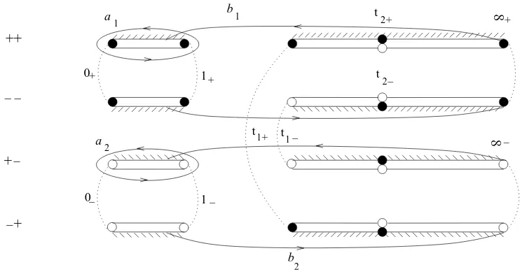
Figure 1. The 4 sheets of C. The segments of two edges of the cuts are glued together if they are: (1) situated one under the other, and (2) hatched by dashes of the same orientation. Thus, the upper edge of the cut on Σ++ betweent1,t2is glued to the lower edge of the cut on Σ−+ betweent1,t2. Four black points over t2 glue together to give one pointt2+∈C, and similarly four white ones givet2−∈C. The 4 preimages of each one of the points 0, 1, t1,∞ are glued in pairs, as shown by the colors black/white and by dotted lines, and give 8 points ofC denoted by 0±, 1±,t1±,∞±.
A=I is the identity matrix, the basisω1, ω2 of Γ(C,Ω1C) and the corresponding period matrix Π0= (I|Z) are called normalized.
The period lattice Λ = Λ(C) is the Z-submodule of rank 4 in Γ(C,Ω1C)∗ generated by the 4 linear forms ω7→R
aiω,ω7→ R
biω. A choice of the basis ωi identifies Γ(C,Ω1C)∗ withC2, and
Λ is then generated by the 4 columns of Π.
The periodZC of C is determined modulo the discrete group Sp(4,Z) acting by symplectic
base changes inH1(C,Z).
Riemann’s bilinear relations. The period matrix of any genus-2 curve C satisfies the conditions
Zt=Z and ℑZ >0.
To determine the periods of bielliptic curves C, it is easier to use the representation from Proposition 1 rather than the standard equation of a genus-2 curve (5). This is due to the fact that we can choose ω1 = dx/y1, ω2 = dx/y2 as a basis of the space Γ(C,Ω1C) of
holo-morphic 1-forms on C, and the periods of these 1-forms are easily related to the periods on Ei. (Basically, (ω1, ω2) can be seen as a basis of eigenvectors of the action of (Z/2Z)2 on C.)
To fix the ideas, we assume for a while that t1, t2 are real and 1 < t1 < t2 (the gen-eral case is obtained by a deformation moving the points ti). Ei can be represented as the
result of gluing two sheets Σi+, Σi−, which are Riemann spheres with cuts along the
seg-ments [0,1] and [ti,∞]. Then C, parameterizing the pairs of points (P1, P2) with Pi ∈ Ei
and with the same x-coordinate, is the result of gluing 4 sheets, which are copies of the Rie-mann sphere with cuts along the segments [0,1] and [t1,∞] labelled by ++, −−, +−, −+. For example, the sheet Σ+− is formed by the pairs (P1, P2) where P1 lies on Σ1+ and P2 on Σ2−. Fig. 1 shows the gluings of the edges of the cuts with the help of hatching and fixes
the choice of the cyclesai,bi. Black points on one vertical are identified, the same for the white
Proposition 3. Let C,E1, E2 be as in Proposition1, and ai, bi as on Fig. 1. Then the period matrix of C is
ZC =
1
2(τ1+τ2) 12(τ1−τ2) 1
2(τ1−τ2) 12(τ1+τ2) !
,
where τi is the period ofEi with respect to the basis γi=πi∗(a1), δi =πi∗(b1) of H1(Ei,Z).
Proof . Letki,libe the periods of the differentialdx/yionEi along the cyclesγi,δirespectively.
Take ωi =πi∗(dx/yi) as a basis of Γ(C,ΩC). We have
Z
a1
πj∗(dx/yj) = Z
πj∗(a1)
dx/yj =kj.
But when calculating the integral overa2, we have to take into account the fact that a positively oriented loop around a cut on Σ+− projects to a positively oriented loop on Σ2−, and the latter defines the cycle −γ2 on E2. Thus π2∗(a2) = −γ2, and the corresponding period acquires an extra sign:
Z
a2
πj∗(dx/yj) = Z
πj∗(a2)
dx/yj = (−1)j+1kj.
The integrals over bj are transformed in a similar way. We obtain the period matrix ofC in the
form
Π =
k1 k1 l1 l1
k2 −k2 l2 −l2
.
Multiplying by the inverse of the left 2×2-block and using the relations τi =li/ki, we obtain
the result.
Corollary 1. The locus H of periods of genus-2 curves C with a degree-2 elliptic subcover is the set of matrices
ZC =
1
2(τ+τ′) 12(τ −τ′) 1
2(τ−τ′) 12(τ +τ′) !
(ℑτ >0,ℑτ′ >0).
Equivalently, H is the set of all the matrices of the form Z =
a b b a
(a, b ∈ C) such that ℑZ >0.
3
Rank-1 connections on
C
and their monodromy
We start by recalling the definition of a connection. LetV be a curve or a complement of a finite set in a curve C. Let E be a vector bundle of rank r ≥ 1 on V. We denote by OV, Ω1
V the
sheaves of holomorphic functions and 1-forms on V respectively. By abuse of notation, we will denote in the same way vector bundles and the sheaves of their sections. A connection on E is aC-linear map of sheaves∇:E→E ⊗Ω1
V which satisfies the Leibnitz rule: for any openU ⊂V,
f ∈ Γ(U,O) and s ∈ Γ(U,E), ∇(f s) = f∇(s) +s df. If E is trivialized by a basis of sections
e = (e1, . . . , er) over U, then we can write ∇(ej) = P
iaijei, and the matrix A(e) = (aij) of
holomorphic 1-forms is called the connection matrix of ∇ with respect to the trivialization e.
If there is no ambiguity with the choice of a trivialization, one can write, by abuse of notation,
Givenr meromorphic sections s= (s1, . . . , sr) which span E over an open subset, the
mat-rix A(s) defined as above is a matrix of meromorphic 1-forms on V. Its poles in V are called apparent singularities of the connection with respect to the meromorphic trivialization s. The
apparent singularities arise at the points P ∈V in which either some of thesi are non-regular,
or all the si are regular but si(P) fail to be linearly independent. They are not singularities of
the connection, but those of the chosen connection matrix.
In the case when the underlying vector bundle is defined not only overV, but over the whole compact Riemann surface C, we can speak about singularities at the points of C \V of the connection itself. To this end, choose local trivializationseP of E at the pointsP ∈C\V, and
define the local connection matrices A(eP) as above, ∇(eP) = ePA(eP). The connection ∇,
regular onV, is said to be meromorphic onCifA(eP) has at worst a pole atP for allP ∈C\V.
If, moreover, A(eP) can be represented in the form A(eP) = B(τP)dτP
τP , where τP is a local
parameter at P and B(τP) is a matrix of holomorphic functions in τP, then P is said to be
a logarithmic singularity of ∇. A connection is called logarithmic, or Fuchsian, if it has only logarithmic singularities.
To define themonodromy of a connection ∇, we have to fix a reference point P0 ∈ V and a basis s = (s1, . . . , sr) of solutions of ∇s = 0, s ∈ Γ(U,E) over a small disc U centered
at P0. The analytic continuation of the si along any loopγ based at P0 provides a new basis
sγ = (sγ
1, . . . , s
γ
r), and the monodromy matrix Mγ is defined by sγ = sMγ. The monodromy
matrix depends only on the homotopy class of a loop, and the monodromy ρ∇ of ∇ is the representation of the fundamental group of V defined by
ρ=ρ∇:π1(V, P0)−→GLr(C), γ 7→Mγ.
Let now C = V be a genus-2 bielliptic curve with an elliptic subcover ϕ : C→E. Our objective is the study of rank-2 connections on E which are direct images of rank-1 connections on C. We first study the rank-1 connections onC and their monodromy representations.
LetLbe a line bundle on C andea meromorphic section of L which is not identically zero. Then a connection ∇L on L can be written as d +ω, where ω is a meromorphic 1-form on C
defined by∇L(e) =ωe. The apparent singularities are simple poles with integer residues at the points whereefails to be a basis ofL. We will start by considering the case whenLis the trivial line bundle O =OC. Then the natural trivialization of L is e= 1, and ω is a regular 1-form. The vector space Γ(C,Ω1C) of regular 1-forms on C is 2-dimensional; letω1,ω2 be its basis. We can write ω=λ1ω1+λ2ω2 withλ1,λ2 inC.
The horizontal sections of O are the solutions of the equation ∇Oϕ = 0. To write down these solutions, we can representC as in Proposition1and introduce the multi-valued functions
z1 = Rω1 and z2 = R ω2, normalized by z1(∞+) = z2(∞+) = 0. We denote by the same symbols z1,z2 the flat coordinates on the JacobianJC =C2/Λ associated to the basis (ω1, ω2) of Γ(C,Ω1
C), and C can be considered as embedded in its Jacobian via the Abel–Jacobi map
AJ :C→JC,P 7−→ ((z1(P), z2(P)) modulo Λ.
To determine the monodromy, we will choose P0 = ∞+ and fix some generators αi, βi of
π1(C,∞+) in such a way that the natural epimorphism
π1(C,∞+)−→H1(C,Z) =π1(C,∞+)/[π1(C,∞+), π1(C,∞+)]
is given by αi7→ai,βi 7→bi.
The following lemma is obvious:
Lemma 1. The general solution of∇Oϕ= 0 is given byϕ=ce−λ1z1−λ2z2, wherecis a complex
constant. The monodromy matrices of ∇O are Mαi = exp(−Haiω), Mβi = exp(− H
biω) (i =
Now we turn to the problem of Riemann–Hilbert type: determine the locus of the represen-tations of Gwhich are monodromies of connections∇L. Since any rank-1 representationρof G
is determined by 4 complex numbers ρ(αi), ρ(βi), we can take (C∗)4 for the moduli space of
representations ofG in which lives the image of the Riemann–Hilbert correspondence.
Before solving this problem on C, we will do a similar thing on an elliptic curve E. The answer will be used as an auxiliary result for the problem onC.
Any rank-1 representation ρ : π1(E)→C∗ is determined by the images ρ(a), ρ(b) of the generatorsa,bof the fundamental group ofE, so that the space of representations ofπ1(E) can be identified withC∗×C∗. We will consider several spaces of rank-1 connections. LetC(E,L) be the space of all the connections ∇ :L→L ⊗Ω1E on a line bundle L on E. It is non empty if only if degL = 0, and then C(E,L) ≃Γ(E,Ω1
E) ≃C. Further, C(E) will denote the moduli
space of pairs (L,∇), that is,C(E) =∪[L]∈J(E)C(E,L). We will also define the moduli spaceC of triples (Eτ,L,∇),C =∪ℑτ >0C(Eτ), and Ctriv =∪ℑτ >0C(Eτ,OEτ), where Eτ =C/(Z+Zτ).
For any of these moduli spaces, we can consider the Riemann–Hilbert correspondence map
RH : (Eτ,L,∇)7−→(ρ∇(a), ρ∇(b)),
where ρ∇ is the monodromy representation of ∇, and (a, b) is a basis of π1(E) corresponding to the basis (1, τ) of the period lattice Z+Zτ. Remark that RH |C(E,L) cannot be surjective by dimensional reasons. The next proposition shows that RH |Ctriv is dominant, though
non-surjective, and thatRH |C is surjective.
Proposition 4. In the above notation,
RH(Ctriv) = (C∗×C∗\ {S1×S1})∪ {(1,1)}, RH(C) =C∗×C∗.
Proof . Let∇= d +ω be a connection on an elliptic curveE, whereω∈Γ(Eτ,Ω1Eτ),A=Haω,
B =H
bω =τ A. By analytic continuation of solutions of the equation ∇ϕ= 0 along the cycles
in E, we obtainρ(a) = e−A and ρ(b) = e−τ A. The pair (−A,−B) = (−A,−τ A) is an element
of (0,0)∪C∗×C∗. By setting z = −A, we deduce RH(Ctriv) = {(ez, ezτ) | (z, τ) ∈ C×H}. The map exp : C∗−→C∗ is surjective, so for all w1 ∈ C∗, we can solve the equation ez = w1, and once we have fixed z, it is possible to solve eτ z = w
2 with respect to τ if and only if (w1, w2)∈/ S1×S1\ {(1,1)}. This ends the proof for RH(Ctriv). The proof forRH(C) is similar to the genus-2 case, see Proposition 5 below.
From now on, we turn to the genus-2 case. We define the moduli spaces C2(C,L), C2(C),
C2, C2,triv similarly to the above, so that C2(C) = ∪[L]∈J(C)C2(C,L), C2 = ∪Z∈HC2(CZ), and Ctriv =∪Z∈HC2(CZ,OCZ). HereH is the locus of periods introduced in Corollary 1,CZ is the
genus-2 curve with period Z, J2(C) = C2/Λ, where Λ ≃ Z4 is the lattice generated by the column vectors of the full period matrix (1|Z) of C. The Riemann–Hilbert correspondence is the map
RH : (CZ,L,∇)7−→(ρ∇(α1), ρ∇(α2), ρ∇(β1), ρ∇(β2))∈(C∗)4,
where the generators αi,βi of π1(C) correspond to the basis of the lattice Λ.
Proposition 5. In the above notation,
RH(C2,triv) =
w∈(C∗)4|(w1w2, w3w4)∈W,
w1
w2
,w3 w4
∈W
,
RH(C2) = (C∗)4,
Proof . Let ∇ = d +ω, ω ∈ Γ(CZ,Ω1CZ). We can consider CZ in its Abel–Jacobi embedding
in JC, then ω = λ1dz1 +λ2dz2, where (z1, z2) are the standard flat coordinates on C2/Λ. Therefore,
RH(CZ,OZ,∇) = eλ1z1, eλ2z2, e
1 2(τ+τ
′
)λ1z1+12(τ−τ′)λ2z2, e12(τ−τ′)λ1z1+12(τ+τ′)λ2z2
.
Denoting the latter 4-vector by w, we see that (w1w2, w3w4) = (ez, eτ z) with z =λ1z1+λ2z2, and (w1
w2,
w3
w4) = (e
z′
, eτ′z′) withz′ =λ1z1−λ2z2.
Then Proposition 4 implies the answer for RH(C2,triv). Now, we will prove the surjectivity of RH |C2. On a genus-2 curve, any line bundle of degree 0 can be represented in the form
L =OC(P1+P2−Q1−Q2) for some 4 points Pi, Qi ∈C. It is defined by its stalks: for any
P ∈C,LP =OP ifP 6∈ {P1, P2, Q1, Q2},LPi = τ1
PiOPi,LQi =τQiOQi, whereτP denotes a local
parameter at P for any P ∈ C. This implies that the constant function e = 1 considered as a section of Lhas simple zeros atPi and simple poles atQi, that is, for its divisor we can write:
(e) = P1+P2−Q1−Q2. According to [2], any line bundle of degree 0 admits a connection, and two connections differ by a holomorphic 1-form. Hence any connection onL can be written in the form ∇=d+ω, ω =ν+λ1dz1+λ2dz2, where ν is a meromorphic 1-form with simple poles at Pi,Qi such that ResPiν = 1, ResQiν =−1 (these are apparent singularities of ∇with
respect to the meromorphic trivialization e= 1).
We can choose the coefficientsλ1,λ2 in such a way thatω will have zero a-periods. Let us denote the periods ofω by Ni:
N1 = Z
a1
ω, N2= Z
a2
ω, N3 = Z
b1
ω, N4 = Z
b2
ω. (6)
Then N1 =N2 = 0 by the choice ofω, and
N2+j = 2πi X
k
Ressk(ω) Z sk
s0
dzj, j= 1,2,
by the Reciprocity Law for differentials of 1st and 3rd kinds [8, Section 2.2], whereP
ksk is the
divisor of poles (ω)∞ of ω, and s0 is any point of C. Taking into account that (ω)∞= (ν)∞=
P1+P2+Q1+Q2, ResPiν= 1, ResQiν=−1, andzj(P) = RP
P0dzj, we can rewrite:
N2+j = 2πi[zj(P1)−zj(Q1) +zj(P2)−zj(Q2)].
Hence the components of the vector 21πi
N3
N4
are the 2 coordinates onJC of the class [L] of
the line bundleL, which is the same as the divisor class [P1+P2−Q1−Q2]. Now, we can finish the proof.
Let (wi)∈(C∗)4. Then, we can find a 1-formη1 of a connection on a degree-0 line bundleL1 with monodromy (1,1, w3, w4) in choosing L1 with coordinates −21πi(logw3,logw4) on JC. In interchanging the roles of a- and b-periods, we will find another 1-form of connection η2 on another degree-0 line bundleL2, with monodomy (w1, w2,1,1). Thenω=η1+η2 is the form of a connection onL1⊗ L2 with monodromy (wi)∈(C∗)4.
4
Direct images of rank-1 connections
We will determine the direct image connections f∗(∇L) = ∇E on the rank-2 vector bundle
want thatE is given the Legendre equationy2 =x(x−1)(x−t),butF6is not so complicated as in (5). Of course, this can be done in many different ways. We will fix forCandf the following choices:
f :C={y2 = (t′−ξ2)(t′−1−ξ2)(t′−t−ξ2)}→E ={y2=x(x−1)(x−t))},
(ξ, y)7→(x, y) = (t′−ξ2, y). (7)
Lemma 2. For any bielliptic curveC with an elliptic subcover f :C→E of degree2, there exist affine coordinates ξ, x, y onC,E such that f,C, E are given by (7) for somet, t′ ∈C\ {0,1},
t6=t′.
Proof . By Proposition 1, it suffices to verify that the two elliptic subcovers E, E′ of the curves C given by (7), as we vary t, t′, run over the whole moduli space of elliptic curves
independently from each other. E′ can be determined from (2). It is a double cover of P1 ramified at t1′, t′1
−1, t′1
−t, ∞. This quadruple can be sent by a homographic transformation to
0, 1, t, t′, hence E′ is given by y2 =x(x−1)(x−t)(x−t′). If we fixt and let vary t′, we will obviously obtain all the elliptic curves, which ends the proof.
The only branch points off inE arep± = (t′,±y0), wherey0= p
t′(t′−1)(t′−t), and thus
the ramification points of f in C are ˜p±= (0,±y0). In particular,f is non-ramified at infinity and the preimage of∞ ∈E is a pair of points∞±∈C. E is the quotient ofCby the involution
ι : C→C, called the Galois involution of the double covering f. It is given in coordinates by
ι: (ξ, y)7→(−ξ, y).
We first deal with the case whenL is the trivial bundleOC, in which we write ∇O instead of ∇L. The direct image E0 = f∗OC is a vector bundle of rank 2 which splits into the direct sum of the ι-invariant and anti-invariant subbundles: E0 = (f∗OC)+ ⊕(f∗OC)−. The latter subbundles are defined as sheaves by specifying their sections over any open subset U of E:
Γ(U,(f∗OC)±) ={s∈Γ(f−1(U),OC) |ι∗(s) =±s}.
Obviously, theι-invariant sections are just functions onE, so the first direct summand (f∗OC)+ is the trivial bundle OE. The second one is generated over the affine set E\ {∞} by a single generator ξ, one of the two coordinates on C. Thus, we can use (1, ξ) as a basis trivializing E0 overE\ {∞}and compute∇=f∗(∇O) in this basis. We use, of course, the constant function 1 to trivialize OC and write ∇O in the form
∇O =d+ω, ω=∇O(1) =λ1dξ
y +λ2 ξdξ
y . (8)
Re-writing∇O(1) =ω in terms of the coordinatex=t′−ξ2, we get:
∇O(1) =−
λ1 2(t′−x)
dx y ξ−
λ2 2
dx y 1.
Likewise,
∇O(ξ) =−
λ1 2
dx y 1−
λ2 2y
dx y ξ−
dx
2(t′−x)ξ.
We obtain the matrix of∇=f∗(∇O) in the basis (1, ξ):
A=
−λ2
2ydx −λ21ydx − λ1
2(t′
−x)ydx −
λ2
2y + 2(t′1 −x)
dx
This matrix has poles at the branch pointsp± with residues
As the sum of residues of a meromorphic 1-form on a compact Riemann surface is zero, we can evaluate the residue at infinity: is a logarithmic connection on a rank-2 vector bundle E0 over E, whose only poles are the two
branch points p± of f. In an appropriate trivialization of E0 over E\ {∞}, ∇ is given by the regularity of ∇overU (the connection matrix of∇in this basis is zero).
We have shown that the only points where the direct image of a regular connection might have singularities are the branch points of the covering. In particular, ∞ is not a singularity of ∇. The fact that the branch points are logarithmic poles follows from the calculation preceding the
statement of the proposition.
At this point, it is appropriate to comment on the horizontal sections of∇, which are solutions
of the matrix ODEdΦ +AΦ = 0 for the vector Φ =
Φ1 Φ2
. We remark that the matrix ODE is
equivalent to one scalar equation of second order which we have not encountered in the literature. It is obtained as follows: the first line of the matrix equation gives
Φ2 =
where Φ1, Φ2 denote the components of a single 2-vector Φ, and the prime denotes the derivative with respect to x. The second equation gives:
Φ′2 = λ1
By substituting here Φ2 in terms of Φ1, we get one second order equation for Φ1. By setting
y2 =P3(x) = x(x−1)(x−t), we have y′ = P
′
3
2y and the differential equation for Φ1 takes the
form
We can also write out the second order differential equation for Φ1 with respect to the flat coordinate z=R dx
an appropriate scaling,x=℘(z) +t+13 ,y = ℘′2(z). Letz0,−z0 be the solutions of℘(z) =t′−t+13 modulo the lattice of periods. Then we have the following equation for Φ1:
Φ′′1+
We now go over to the general case, in whichLis any line bundle of degree 0 on C endowed with a regular connection ∇L. Then f∗L =E is a vector bundle of rank 2 onE endowed with
a logarithmic connection∇E =f∗∇L. We can representLin the formL=O(˜q1+ ˜q2−∞+−∞−) with ˜q1 = (ξ1, y1) and ˜q2 = (ξ2, y2) some points of C. Their images onE will be denoted by qi,
or (xi, yi) in coordinates. We will use 1∈Γ(OC) as a meromorphic trivialization ofL as in the
proof of Proposition5. In this trivialization, the connection form of ∇L has simple poles at the 4 points ˜qi,∞± with residues +1 at ˜qi and −1 at ∞±. It is easy to invent one example of such
y . Hence the general form of∇L is as follows:
∇L= d +ω = d +1 brings us to formulas for the connection ∇E onE. We obtain:
∇L(1) =ω.1 =
Splitting ξ−1ξi into the invariant and anti-invariant parts, we get:
Figure 2. Generators ofπ1(C\ {p˜±},∞+). The parts of the arcs represented in solid (resp. dash) lines are on the upper (resp. lower) sheet.
Remark that the pointsqi =f(˜qi) = (xi, yi) are apparent singularities of∇E. We write down
the residues of A at these points for future use:
Resq1A=
1 2
ξ1
2 1 2ξ1
1 2
!
, Resq2A=
1 2
ξ2
2 1 2ξ2
1 2
!
. (14)
We can also compute Res∞A. First homogenize the equation of E via the change x = x1
x0,
and y = x2
x0. The homogeneous equation is x0x
2
2 = x31 −(1 +t)x21x0+tx1x20. Then, setting
v = x0
x2,u =
x1
x2, we obtain the equation v =u
3−(1 +t)u2v+tuv2 in the neighborhood of ∞. Near ∞= (0,0), we havev∼u3, dyx ∼ −2du. Therefore, Res∞A is:
Res∞A= Resu=0A= −
1 −ξ1+ξ2
2 0 −2
!
. (15)
5
Monodromy of direct image connections
We are using the notation of the previous section. We will calculate the monodromy of the direct image connections ∇E. We will start by choosing generators of the fundamental group
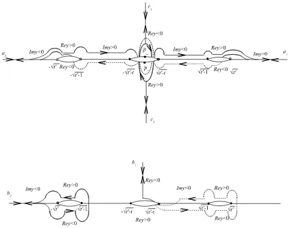
π1(E\{p+, p−}). To express the monodromy of∇in terms of periods ofC, we will first introduce generators ai,bi,ci forπ1(C\ {p˜+,p˜−}), and then descend some of them to E by applying f∗.
that t, t′ are real and 1 < t < t′ (for general t, t′, the loops ai, bi, ci are defined up to an
isotopy bringingt,t′ onto the real axis so that 1< t < t′). C can be represented as the result of
gluing two copies of the Riemann sphere along three cuts. We call these copies of the Riemann sphere upper and lower sheets, and the cuts are realized along the rectilinear segments [−√t′, −√t′−1], [−√t′−t,√t′−t] and [√t′−1,√t′]. The sheets are glued together in such a way
that the upper edge of each cut on the upper sheet is identified with the lower edge of the respective cut on the lower sheet, and vice versa. Let ∞+ be on the upper sheet, singled out by the condition ℑy >0 when ξ ∈ R, ξ → +∞. This implies that the values of ℜy,ℑy on R are as on Fig. 2, where the loopsai,bi,ci generatingπ1(C\ {p˜+,p˜−}) are shown. Remark that the loopsciare chosen in the formci=di˜cid−i 1, wherediis a path joining∞+ with some point close to ˜p± and ˜ci is a small circle around ˜p± (the valuesi= 1,2 correspond to ˜p+, ˜p− respectively).
The paths di follow the imaginary axis of the upper sheet.
Now, we go over to E. Set a = f∗(a1), b = f∗(b1), and define the closed paths running round the branch pointsp±as follows: γi=f(di)˜γif(di)−1, where ˜γi are small circles aroundp±
running in the same direction as f(˜ci) (but f(˜ci) makes two revolutions around p±, whilst ˜γi
only one).
One can verify that the thus defined generators of both fundamental groups satisfy the relations [a1, b1]c1[a2, b2]c2 = 1 and [a, b]γ1γ2 = 1 and that the group morphism
f∗ :π1(C\ {p˜±},∞+)−→π1(E\ {p±},∞) is given by the formulas
f∗(a1) =a, f∗(b1) =b, f∗(a2) =γ1−1aγ1, f∗(b2) =γ1−1bγ1, f∗(ci) =γ2i (i= 1,2).
As∇Lis regular at ˜p±, it has no monodromy alongci, and this together with the above formulas
forf∗ immediately implies that the monodromy matricesMγi of∇E are of order 2.
We first assume thatL=OC is trivial, in which case ∇L is denoted∇O, and∇E just∇. As
in the previous section, we trivializeE0=f∗(OC) by the basis (1, ξ) overE\ {∞}. Splitting the
solutionϕ=e−λ1z1−λ2z2 of∇Oϕ= 0 into theι-invariant and anti-invariant parts, we representϕ
by a 2-component vector in the basis (1, ξ):
Φ = e
−λ2z2cosh(λ
1z1)
−e−λ2z2
ξ sinh(λ1z1) !
.
We have to complete Φ to a fundamental matrix Φ, and then we can define the mon-odromy Mγ along a loop γ by Tγ(Φ) = ΦMγ, where Tγ denotes the analytic continuation
along γ. We already know the first column of Φ: this is just Φ. Denote it also by Φ1, the column vector
Φ1,1 Φ2,1
. It remains to find Φ2 =
Φ1,2 Φ2,2
so that
Φ=
Φ1,1 Φ1,2 Φ2,1 Φ2,2
is a fundamental matrix. By Liouville’s theorem, the matrix equation Φ′+AΦ= 0 implies the
following scalar equation for Ψ = det Φ: Ψ′+ Tr (A)Ψ = 0. In our case, Tr (A) =−λ2
y −
1 2(t′
−x), and we get a solution in the form: Ψ = e√−2λ2z2
t′ −x =
e−2λ2z2
ξ . Thus we can determine Φ2 from the
system:
cosh(λ1z1)Φ2,2+ 1
ξ sinh(λ1z1)Φ1,2=
e−2λ2z2
ξ ,
Φ′1,2 = 1
Eliminating Φ2,2, we obtain an inhomogeneous first order linear differential equation for Φ1,2.
represent the result in a form, in which the real and imaginary parts of all the entries are visible as soon as t, t′ ∈ R and 1 < t < t′. Under this assumption, the entries of the period matrix Π = ((aij|(bij) ofCare real or imaginary and can be expressed in terms of hyperelliptic integrals
along the real segments joining branch points.
Thus reading the cycles of integration from Fig.2, we obtain:
a1,1=−a1,2 = 2iK, K=
Proposition 8. The monodromy matrices of the connection ∇ = f∗(∇O), where ∇O is the rank-1 connection (8), are given by
Now we turn to the general case of nontrivialL. Our computations done in the special case allow us to guess the form of the fundamental matrix of solutions to∇EΦ = 0, where∇E =f∗∇L
and ∇L is given by (11) (remark, it would be not so easy to find it directly from (12)):
Proposition 9. The monodromy matrices of the connection∇E given by (12) are the following:
Proof . By a direct calculation using the observation that the periods of ω∗ are (N2, N1, N4,
N3).
Here the connection (12) depends on 6 independent parameters ˜q1, ˜q2, λ1, λ2, t, t′, and the monodromy is determined by the 4 periods Ni. Hence, it is justified to speak about the
isomonodromic deformations for this connection. The problem of isomonodromic deformations is easily solved upon an appropriate change of parameters. Firstly, change the representation of ω: writeω=ω0+λ1ω1+λ2ω2, whereω0 =ν+λ10ω1+λ02ω2 is chosen with zeroa-periods, as in the proof of Proposition 5, and assume that (ω1, ω2) is a normalized basis of differentials of first kind on C. Secondly, replace the 2 parameters ˜q1, ˜q2 by the coordinates z1[L], z2[L] of the class of L =O(˜q1 + ˜q2− ∞+− ∞−) in JC. Thirdly, replace (t, t′) by the periodZ of C. Then an isomonodromic variety Ni = const (i= 1, . . . ,4) is defined, in the above parameters,
by the equations
λ1
λ2
= const,
z1[L]
z2[L]
+Z
λ1
λ2
= const.
Thus the isomonodromy varieties can be considered as surfaces in the 4-dimensional relative Jacobian J(C/H) of the universal family of bielliptic curves C→H over the bielliptic period locus H introduced in Corollary 1. The fiber CZ of C over a point Z ∈ H is a genus-2 curve
with period Z, and J(C/H)→H is the family of the Jacobians of all the curves CZ as Z runs
over H. The isomonodromy surfaces Sλ1,λ2,µ1,µ2 in J(C/H) depend on 4 parameters λi, µi.
Every isomonodromy surface is a cross-section of the projection J(C/H)→H defined by
Sλ1,λ2,µ1,µ2 =
(Z,[L])|Z ∈ H, [L]∈JCZ,
z1[L]
z2[L]
=−Z
λ1
λ2
+
µ1
µ2
.
6
Elementary transforms of rank-2 vector bundles
In this section, we will recall basic facts on elementary transforms of vector bundles in the particular case of rank 2, the only one needed for application to the underlying vector bundles of the direct image connection in the next section. The impact of the elementary transforms is twofold. First, they provide a tool of identification of vector bundles. If we are given a vector bundleEand if we manage to find a sequence of elementary transforms which connectEto some “easy” vector bundleE0 (likeO ⊕ O(−p) for a pointp), we provide an explicit construction ofE and at the same time we determine, or identifyE via this construction. Second, the elementary transforms permit to change the vector bundle endowed with a connection without changing the monodromy of the connection. The importance of such applications is illustrated in the article [7], in which the authors prove that any irreducible representation of the fundamental group of a Riemann surface with punctures can be realized by a logarithmic connection on a semistable vector bundle of degree 0 (see Theorem 2). On one hand, this is a far-reaching generalization of Bolibruch’s result [1] which affirms the solvability of the Riemann–Hilbert problem over the Riemann sphere with punctures, and on the other hand, this theorem gives rise to a map from the moduli space of connections to the moduli space of vector bundles, for only the class of semistable vector bundles has a consistent moduli theory. We will illustrate this feature of elementary transforms allowing us to roll between stable, semistable and unstable bundles in the next section.
Let E be a curve. As before, we identify locally free sheaves on E with associated vector bundles. Let E be a rank-2 vector bundle on E, p a point of E, E|p = E ⊗Cp the fiber of E
at p. Here Cp is the sky-scraper sheaf whose only nonzero stalk is the stalk at p, equal to the
to be confused with the stalk Ep of E at p, the latter being a free Op-module of rank 2. Let
e1, e2 be a basis of E|p. We extende1, e2 to sections of E in a neighborhood of p, keeping for them the same notation. We define the elementary transforms E+ and E− of E as subsheaves
of E ⊗C(E)≃C(E)2, in giving their stalks at all the points of E:
E−=elm−p,e2(E), Ep−=OpτPe1+Ope2,
E+=elm+p,e1(E), Ep+=Op 1
τP
e1+Ope2, (16)
Ez±=Ez, ∀z∈E\ {p},
where τP denotes a local parameter at p. The thus obtained sheaves are locally free of rank 2.
They fit into the exact triples:
0→E−→E γ //C(p)→0, 0→E→E+→C(p)→0. (17)
Remark, that the surjection γ restricted to E|p is a projection parallel to the e2 axis; this is the reason for which we included in the notation ofelm− its dependence one2. Thus, if we varye1, in keeping e2 (or in keeping the proportionality class of e2), the isomorphism class of elm−e2
will not change, but it can change if we vary the proportionality class [e2] in the projective line P(E|p).
For degrees, we have degE±= degE ±1. We can give a more precise version of this equality in terms of the determinant line bundles: detE± = detE(±p). Here and further on, given
a line bundle L and a divisor D = P
nipi on E, we denote by L(D) (“L twisted by D”) the
following line bundle, defined as a sheaf by its stalks at all the points of E: L(D)z = Lz
if z is not among the pi, and L(D)pi = τpi−niLz. For example, the regular sections of L(p)
can be viewed as meromorphic sections of L with at most simple pole at p, whilst the regular sections of L(−p) are regular sections of L vanishing at p. For the degree of a twist, we have degL(D) = degL+ degD= degL+P
ni, so that degL(±p) = degL ±1.
A similar notion of twists applies to higher-rank bundlesE: the twist E(D) can be defined either as E ⊗ O(D), or via the stalks in replacingL by E in the above definition. For degrees, we have degE(D) = degE+ rkE ·degD. Coming back to rkE = 2 and twisting E by ±p, we obtain some more exact triples:
0→E+→E(p)→C(p)→0, 0→E(−p)→E−→C(p)→0.
They are easily defined via stalks, as E(p) = E ⊗ OE(p) is spanned by τP1 e1, τP1 e2 at p, and
E(−p) byτPe1,τPe2.
A basis-free description of elms can be given as follows: Let W ⊂ E|p be a 1-dimensional vector subspace. Then elm−(p,W)(E) is defined as the kernel of the composition of natural maps
E→E|p→E|p/W (here E|p,E|p/W are considered as sky-scraper sheaves, i.e. vector spaces placed
atp). The positive elm is defined via the duality:
elm+p,W(E) := (elm−p,W⊥(E∨))∨.
To set a correspondence with the previous notation, we write:
elm+p,e1(E) =elm+p,Ce
1(E), elm
−
p,e2(E) =elm−p,Ce2(E).
One can also define elm+ as an appropriateelm−, applied not toE, but toE(p):
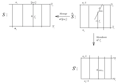
Figure 3. Decomposition ofelm−
in a blowup followed by a blowdown.
We will now interpret the elementary transforms in terms of ruled surfaces. For a vector bundle E over E, we denote by P(E) the projectivization of E, whose fiber over z ∈ E is the projective lineP(E|z) parameterizing vector lines inE|z. It has a natural projectionP(E)→Ewith fibers isomorphic toP1 and is therefore called a ruled surface. We will see that the elementary transforms of vector bundles correspond to birational maps between associated ruled surfaces which split into the composition of one blowup and one blowdown. The transfer to ruled surfaces allows us to better understand the structure of E, for it replaces all the line subbundlesL ⊂ E
by cross-sections of the fiber bundleP(E)→E; the latter cross-sections being curves in a surface, we can use the intersection theory on the surface to study them. As an example, we will give a criterion of (semi)stability of E in terms of the intersection theory onP(E).
Let us return to the setting of the description of elms via bases. We can assume that e1,
e2 are rational sections of E, regular and linearly independent at p. Let S = P(E) and let
π :S−→E be the natural projection. Then e1, e2 define two global cross-sections of π, which will be denoted e1, e2. If E− = elm−p,e2(E), then the natural map E−−→E gives rise to the
birationnal isomorphism of ruled surfacesS−→S−=P(E−) which splits into the composition of
one blowup and one blowdown, as shown on Fig. 3.
Let fp denote the fiber π−1(p) ≃ P1 of π; we keep the same notation for curves and their
proper transforms in birational surfaces. We label some of the curves by their self-intersection; for example, (e12)S =α1, (fp2)S = 0, (fp2)Sˆ = −1. For any vector v ∈ E|p\ {0}, we denote by
[p, v] the point of fp = P(E|p) which is the vector line spanned by v. Remark that the
cross-sections e1, e2 are disjoint in the neighborhood of p where e1, e2 is a basis of E, but e1 can intersecte2 at a finite number of points wheree1,e2 fail to generate E.
The positiveelm has a similar description. Basically, as P(E)≃P(E ⊗L) for any invertible sheaf L on E, we have P(E) ≃P(E(p)). Hence, in view of (18),elm+ and elm− have the same
representation on the level of ruled surfaces. There exists also an elegant way to defineelm− in using π :S−→E:
Here, IS,[p,v] is the ideal sheaf of the point [p, v], and F(1) denotes the twist of a sheaf F by
OP(E)/E(1). We have the natural exact triple of an ideal sheaf on S=P(E):
0→IS,[p,v](1)→OS/E(1)→C[p,v]→0.
By a basic property of the tautological sheaf OS/E(1), we have π∗OS/E(1)≃ E. By applyingπ∗, we get the exact triple
0→π∗IS,[p,v](1)→E→Cp→0.
One can prove that in this way we recover the first exact triple (17).
Now, we will say a few words about the (semi)-stability in terms of ruled surfaces.
Definition 3. A rank-2 vector bundle on a curve E is stable (resp. semistable) if for any line subbundle L ⊂ E, degL< 12degE (resp., degL ≤ 1
2degE), or equivalently, if for any surjection
E→M onto a line bundle M, degM > 12degE (resp., degM ≥ 12degE). A vector bundle is called unstable if it is not semistable. It is called strictly semistable if it is semistable, but not stable.
Definition 4. Let E be a rank-2 vector bundle on a curve E. The index of the ruled surface
π :S=P(E)−→E is the minimal self-intersection number of a cross-section of π:
i(S) = min{(e)S2 |e⊂S is a cross-section ofπ}.
The assertion of the following proposition is well-known, see e.g. [14, p. 55]. For the reader’s convenience, we provide a short proof of it.
Proposition 10. E is stable (resp. semi-stable) iff i(S)>0 (resp. i(S)≥0).
Proof . The cross-sections of P(E)−→E are in 1-to-1 correspondence with the exact triples
0→L1 α //E
β
/
/L
2→0, (19)
whereL1,L2 are line bundles overE. The cross-sectioneassociated to such a triple isP(L1)⊂ P(E). It is the zero locus of π∗β ◦π∗α ∈ Hom(π∗L1, π∗L2) ≃ H0(S, π∗(L2 ⊗ L−1
1 )). Hence, the normal bundle Ne/S is isomorphic to L2 ⊗ L−11. The stability (resp. semi-stability) of E is equivalent to the fact that degL1 < degL2 (resp. degL1 ≤ degL2) for any triple (19). As (e2)S= degNe/S = degL2−degL1, this ends the proof.
We will end this section by two lemmas which help to identify vector bundles via the geometry of the associated ruled surfaces.
Lemma 3. Let E be a rank-2 vector bundles over a curve X such that the associated ruled surface S = P(E) has two disjoint cross-sections s1, s2. Then E =L1⊕ L2, where Li are line
subbundles of E corresponding to si: si = P(Li), i = 1,2. Further, for the self-intersection numbers of si, we have (s1)2=−(s2)2= degL2−degL1.
Proof . The first assertion is obvious, and the second one follows from the formula for (e2)S in
the proof of Proposition 10, in taking into account thatE =L1⊕ L2 fits into an exact triple of
the form (19).
Lemma 4. Let E be a rank-2 vector bundle over a curve X, L a line subbundle of E and
s = P(L) the associated cross-section of the ruled surface S = P(E). Let p ∈ X, [p, v] ∈ fp, where fp denotes the fiber of S over p. Let S± = P(E±), where E± = elm±p,v, π± : S 99K S± the natural birational map, s± the proper transform of sinS± underπ± (that is, the closure of
(i) If[p, v]∈s, then(s±)2S± = (s2)S−1,degL+= degL+ 1, and degL−= degL. Moreover, L+ ≃ L(p) and L−≃ L.
(ii) If[p, v]6∈s, then(s±)2
S± = (s2)S+ 1,degL+= degL, and degL−= degL −1. Moreover, L+ ≃ Land L−≃ L(−p).
Proof . The formulas for (s±)2S± follow from the behavior of the intersection indices as shown
on Fig. 3, and those for degL± are easily deduced directly from the definition of elementary
transforms (16) by choosing fore1 ore2 a rational trivialization ofL.
7
Underlying vector bundles of direct image connection
Let us go over again to the setting of Section 4. Consider first the case whenL is the trivial bundle,L=OC. The following fact is well known:
Lemma 5. Letf :X→Y be a finite morphism of smooth varieties of degree2and∆the class of its branch divisor in Pic(Y). Then ∆is divisible by two in Pic(Y), and there exists δ⊂Pic(Y)
such that 2δ is linearly equivalent to ∆and f∗OX =OY ⊕ OY(−δ).
Proof . See [11, Section 1].
Applying this lemma tof :C→E, we find thatf∗OC =OE⊕ OE(−δ), where 2δ≃p++p−.
This property determinesδ only moduloE[2], but as we saw in Section4,OE(−δ) is trivialized by a sectionξ overE\ {∞}, thusδ=∞and f∗OC =OE⊕ OE(−∞). We deduce:
Proposition 11. If L = OC, then the direct image connection ∇E = f∗(∇L), determined by formula (12), is a logarithmic connection on the vector bundle E0 = OE ⊕ OE(−∞) with two
poles at p+, p−.
Let now L be an arbitrary line bundle over C of degree 0. By continuity, degf∗L = degf∗OC =−1. To determine f∗L, we use the following lemma:
Lemma 6. Let X be a nonsingular curve, p a point in X, and z a local parameter at p. Let E be a rank-2 vector bundle on X with a meromorphic connection ∇, regular at p. Let s1, s2
be a pair of meromorphic sections of E, linearly independent over C(X) and F = hs1, s2i the
subsheaf ofE ⊗C(X) generated bys1,s2 as aOX-module. LetAbe the matrix of ∇with respect
to the C(X)-basis s1, s2 and A = resz=0A. Assume that E|p has a basis v1, v2 consisting of
eigenvectors of A. Then v1, v2 extend to a basis of the stalk Ep, the corresponding eigenvalues
n1, n2 of A are integers and we have the following relations between the stalks of subsheaves of
E ⊗C(X) atp:
Ep=hv1, v2i, Fp =hzn1v1, zn2v2i, if n1= 1, n2 = 0, Ep =elm+p,v1(Fp),
if n1=−1, n2 = 0, Ep =elm−p,v2(Fp),
if n1=n2, Ep = (F(n1))p.
Proof . Straightforward.
Let us apply this lemma to the connection∇E, given by formula (12) in the basis (1, ξ). We have: Ep 6=Fp ⇐⇒ p∈ {q1, q2,∞},
Ai = ResqiA=
1 2
ξ1
2 1 2ξ1
1 2
!
(i= 1,2), A∞= Res∞A=
−1 −ξ1+ξ2
2 0 −2
We list the eigenvectors vj(i),vj(∞) together with the respective eigenvalues for the matricesAi,
A∞:
v1(i)=
−ξi
1
, η1i = 0, v2(i) =
ξi −1
, η2i =−1,
v(1∞)=
1 0
, η1∞= 1, v2(∞)=
−ξ1+ξ2
2 1
, η2∞=−2.
Applying Lemma6(twice at ∞), we obtain the following corollary:
Corollary 2. Let L = OC(˜q1 + ˜q2 − ∞+− ∞−), q˜i = (ξi, yi), qi = f(˜qi), i = 1,2, as in Proposition 7, and letvj(i) be the eigenvectors of Ai as above. Then
E =elm+
q1,v(1)2
elm+
q2,v(2)2
(E0(−∞)).
Remark 1. Note that though the sheaf-theoretic direct image f∗L does not depend on the choice of a connection∇L on L, our method of computation off∗L, given by Corollary2, uses the direct image connection ∇E =f∗∇L for some∇L.
Proposition 12. For genericL ∈Pic(C), the rank-2 vector bundle E is stable.
Proof . Starting from the ruled surface S0 = P(E0) = P(OE ⊕ OE(−∞)), we apply two ele-mentary transforms S0→S1→S2=P(E), and we have to prove that any cross-section of S2 has strictly positive self-intersection, provided that ˜qi = (ξi, yi) are sufficiently generic. For a
ratio-nal sectionsofE0, let us denote bysthe associated cross-section ofS0. S0is characterized by the existence of two distinguished sectionss1,s2 associated tos1 = 1,s2=ξ with self-intersections
s21 =−1, s22 = 1, and we have the relations s1s2 = 0, s2 ∼ s1+f∞, where fp = π−1(p) is the
fiber of the structure projectionπ:S0−→E. When there is no risk of confusion, we will keep the same notation for curves and their proper transforms in birational surfaces. Any cross-sections
is linearly equivalent to s1 +fp1 +· · ·+fpr for some points p1, . . . , pr in E, and s2 = 2r+ 1.
In particular, i(S0) =−1, attained on s1. Remark that s0 is rigid, whilst s1 moves in a pencil
|s1+f∞|. Let us applyelm+
q1,v2(1)
. First, we blow upP1= [q1, v(1)2 ]. Let e1 be the corresponding
(−1)-curve and ˆS0 the blown up surface. For the self-intersection numbers of the cross-sections, we have the following relations: (s2)
ˆ
S0 = (s
2)
S0 if P1 ∈/ s and (s2)Sˆ0 = (s
2)
S0 −1 if P1 ∈ s.
Hence, ˆS0 has only one cross-section for each one of the self-intersection numbers −1, 0, and (s2)S0 ≥1 for all the other cross-sections. The cross-section with self-intersection−1 is s1 and
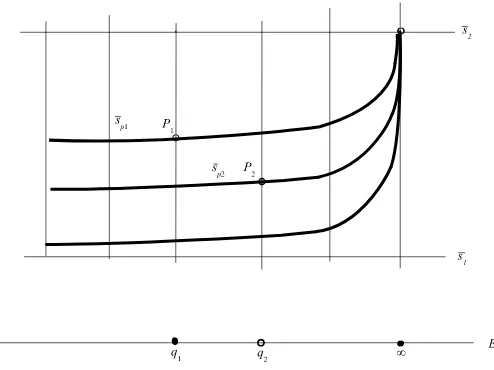
the one with self-intersection 0 is the proper transform of the unique member sP1 of the pencil
| s1 +f∞ | on S0 going through P1, see Fig. 4. The next step is the blowdown of fq1 ⊂ Sˆ0.
The self-intersection number of all the cross-sections of ˆS0→E that meetfq1 goes up by 1. We
conclude that S1 =P(elm+q1,v1
2(E0)) has two cross-sectionssP1,s1 with square 0, and (s
2)
S1 ≥2
for any other cross-section of S1. In the language of vector bundles, this means that E1 is the direct sum of two line bundles of degree 0. More precisely, E1 =OE⊕ OE(q1− ∞) by Lemma 3, the first summand corresponding to s1 and the second one to sP1.
The second elementary transform is performed atP2 ∈S1. AsP2 ∈/sP1∪s1, the minimal
self-intersection number of a cross-section inS1 passing throughP2 is 2. The elementary transform decreases by 1 the self-intersection of such cross-sections and increases by 1 the self-intersection of all other cross-sections (Lemma4). Hence,i(S2) = 1, the value attained on many cross-sections, for example, sP2,sP1,s1. This ends the proof.
Figure 4. The ruled surface S0. The pencil| s1+f∞ | has a unique member passing throughPi for eachi= 1,2.
Using Atiyah’s theorem in our case, we have degN =−1 , so that N can be represented in the form N = OE(−q) for some q ∈ E. E is obtained as the unique non-trivial extension of vector bundles:
0→OE(−q)→E→OE→0.
Moreover, the correspondence E ↔ q identifies the moduli space Ms
E(2,−1) of rank-2 stable
vector bundles of degree −1 overE withE itself. We deduce:
Corollary 3. Under the above identification Ms
E(2,−1)≃E, the rational map:
f :JC 99KMsE(2,−1),
L=OC( ˜q1+ ˜q2− ∞+− ∞−)7→f∗(L)
can be given by
[ ˜q1+ ˜q2− ∞+− ∞−]7→[q1+q2−2∞].
Now we go over to the nongeneric line bundlesL. The direct imagef∗L can be unstable for specialL. This may happen when either the argument of Proposition12does not work anymore, or when formulas (12)–(15) are not valid. We list the cases which need a separate analysis in the next proposition.
Proposition 13. LetL=OC( ˜q1+ ˜q2−∞+−∞−),E =f∗(L),E0 =f∗OC, as above. Whenever ˜
qi is finite, it will be represented by its coordinates: q˜i = (ξi, yi). The following assertions hold:
(a) If q˜1+ ˜q2 is a divisor in the hyperelliptic linear seriesg21(C) (that isξ1 =ξ2, y1 =−y2, or
{q˜1,q˜2}={∞+,∞−}), then E ≃ E0, and henceE is unstable.
(b) If q˜1= ˜q2 6=∞±, then E ≃ OE(−∞)⊕ OE(2q1−2∞) is unstable.
(c) If q˜i=∞± for at least one value i∈ {1,2}, then E ≃ OE(−2∞+q3−i)⊕ OE is unstable.
(d) If q˜i = ˜p± for exactly one value i ∈ {1,2}, then E is a stable bundle of degree −1 with
Proof . (a) In this case, sp1 =sp2, ˜q1+ ˜q2∼ ∞++∞−, thenL ≃ OC, andE ≃ E0. (12)–(15). We obtain the following residues:
Resp±A=
As in the proof of Proposition12, we can describe E as the result of two successive positive elm’s applied to E0(−∞). In contrast to the general case, considered in Lemma 6, the second elm has for its center the point ˜P1 = sP1 ∩f˜q1 ⊂S1, where ˜fq1 is the fiber of S1→E over q1.
As (sP1)2S1 = 0, the resulting surface S2 has a cross-section with self-intersection −1, thus
i(S2) =−1, and consequently E is unstable. Applying Lemmas 3and 4, we can identify it with
OE(−∞)⊕ OE(2q1−2∞).
(c) Let, for example, ˜q2=∞−. ThenLdegenerates toOC( ˜q1− ∞+), and we can again write the connection in the same way as in the previous case. E is obtained fromE0(−∞) by 2 positive elms. From Lemmas 3and 4, we deduce that E ≃ OE(−2∞+q1)⊕ OE. second one transforms E1 into a stable vector bundleE2 which fits into the exact triple
0→OE→E2→OE(q1+p+− ∞)→0.
Thus, the resulting vector bundle E =f∗(L) = E2(−∞) behaves exactly as in the general case
Next we will discuss Gabber’s elementary transforms as defined by Esnault and Viehweg [7]. Gabber’s transform of a pair (E,∇), consisting of a vector bundleEover a curve and a logarithmic connection onE is another pair (E′,∇′), whereE′ is an elementary transform ofE at some polep
of∇, and one of the eigenvalues of Resp∇′differs by 1 from the respective eigenvalue of Resp∇,
whilst the other eigenvalues as well as the other residues remain unchanged. We adapt the definition of Esnault–Viehweg to the rank-2 case and to our notation:
Definition 5. LetE be a rank-2 vector bundle on a curveX,∇a logarithmic connection onE,
p∈X a pole of∇, and v∈ E|p an eigenvector of the residue Resp(∇)∈End(E|p). The Gabber
transformelmp,v(E,∇) is a pair (E′,∇′) constructed as follows:
(i) E′ =elm+
p,v(E).
(ii) ∇′ is identified with∇under the isomorphismE|X
−p≃ E′|X−p as a meromorphic
connec-tion over X−p, and this determines ∇′ as a meromorphic connection over X.
By a local computation of∇′ atp one proves:
Lemma 7. In the setting of Definition 5, let us complete v to a basis (e1 =v, e2) of E near p,
so that Ep′ = Op· τp1v+Op·e2 and the matrix R of Resp(∇) has the form R =
λ1 ∗ 0 λ2
.
Then ∇′ is a logarithmic connection on E′ and the matrix R′ of its residue atp computed with
respect to the basis (e′
1, e′2) = (τpv, e2) of E′ has the form R′ =
λ1−1 0
∗ λ2
.
Theorem 2 (Bolibruch–Esnault–Viehweg [1, 7]). Let E be a rank-r vector bundle on a curve X, ∇ a logarithmic connection on E, and assume that the pair (E,∇) is irreducible in the following sense: E has no ∇-invariant subbundles F ⊂ E. Then there exists a sequence of Gabber’s transforms that replaces (E,∇) by another pair (E′,∇′), in whichE′ is a semistable vector bundle of degree 0and∇′ is a logarithmic connection onE′ with the same singular points and the same monodromy as ∇.
We are illustrating this theorem by presenting explicitly one elementary Gabber’s transform which transforms our bundleE =f∗Lof degree −1 into a semistable bundleE′ of degree 0:
Proposition 14. Let E, ∇ be as in Proposition 12. Let v be an eigenvector of Resp+(∇)
with eigenvalue 12 (see formula (13)). Then the Gabber transform (E′,∇′) = elm+
p+,v(E,∇)
satisfies the conclusion of the Bolibruch–Esnault–Viehweg theorem: E′ is semistable of degree 0 and ∇′ is a logarithmic connection with the same singularities and the same monodromy as ∇. Furthermore, E′ ≃ OE(p+− ∞)⊕ OE(q1+q2−2∞).
Proof . By Corollary 2, E′ is the result of application of three positive elms to E0(−∞) = OE(−∞)⊕ OE(−2∞):
E′ =elm+p+,velm+
q1,v(1)2
elm+
q2,v(2)2
(E0(−∞)).
The surface S0 =P(E0(−∞)) can be decomposed as the open subsetS0\s1 (see Fig. 4), which is a line bundle over E with zero section s2, plus the “infinity section” s1. The line bundle is easily identified as the normal bundle to s2 in S0: S0\s1 ≃ Ns2/S0 ≃ OE(∞). Then the
pencil |s2| = |s1 +f∞| is the projective line which naturally decomposes into the affine line
H0(E,O(∞)) and the infinity point representing the reducible member of the pencil s1+f∞
(the curves sP1, sP2 shown on Fig. 4 are members of this pencil). The fact that all the global