El e c t ro n ic
Jo ur
n a l o
f P
r o
b a b il i t y
Vol. 13 (2008), Paper no. 64, pages 1952–1979. Journal URL
http://www.math.washington.edu/~ejpecp/
Positively and negatively excited random walks on
integers, with branching processes
Elena Kosygina
∗Department of Mathematics Baruch College - CUNY One Bernard Baruch Way New York, NY 10010, USA [email protected]
Martin P.W. Zerner
Mathematisches Institut Universität Tübingen Auf der Morgenstelle 10 72076 Tübingen, Germany [email protected]
Abstract
We consider excited random walks onZwith a bounded number of i.i.d. cookies per site which may induce drifts both to the left and to the right. We extend the criteria for recurrence and transience by M. Zerner and for positivity of speed by A.-L. Basdevant and A. Singh to this case and also prove an annealed central limit theorem. The proofs are based on results from the literature concerning branching processes with migration and make use of a certain renewal structure.
Key words: Central limit theorem, excited random walk, law of large numbers, positive and negative cookies, recurrence, renewal structure, transience.
AMS 2000 Subject Classification:Primary 60K35, 60K37, 60J80.
Submitted to EJP on January 13, 2008, final version accepted October 14, 2008.
1
Introduction
We consider nearest-neighbor random walks on the one-dimensional integer lattice in an i.i.d. cookie environment with a uniformly bounded number of cookies per site. The uniform bound on the number of cookies per site will be denoted by M ≥ 1, M ∈ N. Informally speaking, a cookie
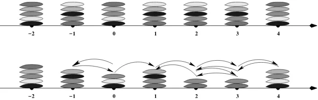
environment is constructed by placing a pile of cookies at each site of the lattice (see Figure 1). The piles of cookies represent the transition probabilities of the random walker: upon each visit to a site the walker consumes the topmost cookie from the pile at that site and makes a unit step to the right or to the left with probabilities prescribed by that cookie. If the cookie pile at the current site is empty the walker makes a unit step to the right or to the left with equal probabilities.
−2 −1 0 1 2 3 4
−2 −1 0 1 2 3 4
Figure 1: The top picture is an example of an i.i.d. cookie environment withM =5, which consists of two types of cookie piles. An independent toss of a fair coin determines which type of cookie pile is placed at each site of the lattice. Various shades of gray allude to different transition probabilities associated to different cookies. The bottom picture shows the first few possible steps of a random walker in this cookie environment starting at 0.
A cookie will be called positive (resp. negative) if its consumption makes the walker to go to the right with probability larger (resp. smaller) than 1/2. A cookie which is neither positive nor negative will be called a placebo. Placebo cookies allow us to assume without loss of generality that each pile originally consists of exactlyM cookies. Unless stated otherwise, the random walker always starts at the origin.
The term “excited random walk" was introduced by Benjamini and Wilson in[BW03], where they considered random walks onZd, d ≥1, in an environment of identical cookies, one per each site.
Allowing more (or fewer) than one cookie per site and randomizing the environment naturally gave rise to the multi-excited random walk model in random cookie environments. We refer to[Zer05]
and [Zer06] for the precise description and first results. It was clear then that this new model exhibits a very interesting behavior for d =1. We shall mention some of the results for d ≥ 2 in Section 9 and now concentrate on the one-dimensional case.
The studies of excited random walks on integers were continued in [MPV06], [BS08a], and
[BS08b]. [AR05]deals with numerical simulations of this model. In all papers mentioned above a (possible) bias introduced by the consumption of a cookie was assumed to be only in one direction, say, positive. The recurrence and transience, strong law of large numbers [Zer05], conditions for positive linear speed[MPV06],[BS08a], and the rates of escape to infinity for transient walks with zero speed[BS08b]are now well understood. Yet some of the methods and facts used in the proofs (for example, comparison with simple symmetric random walks, submartingale property) depend significantly on this “positive bias” assumption.
are the recurrence/transience criterion (Theorem 1), the criterion for positive linear speed (Theo-rem 2) and an annealed central limit theo(Theo-rem (Theo(Theo-rem 3). The first two theo(Theo-rems are extensions of those for non-negative cookie environments but we believe that this is a purely one-dimensional phenomenon. Moreover, in Section 9 we give an example, which shows that, at least ford≥4, the criteria for recurrence or transience and for positive linear speed can not depend just on a single parameter, the average total drift per site (see (3)). The order of the cookies in the pile should matter as well.
The proofs are based on the connections to branching processes with migration. Branching pro-cesses allowing both immigration and emigration were studied by several authors in the late 70-ties through about the middle of the 90-ties, and we use some of the results from the literature (Sec-tion 2). See the review paper [VZ93] for more results and an extensive list of references up to about 1990. The connection between one-dimensional random walks and branching processes was observed long time ago. In particular, it was used for the study of random walks in random environ-ments, see e.g.[KKS75]. In the context of excited random walks, this idea was employed recently in [BS08a], [BS08b](still under the “positive bias” assumption). In the present paper we are us-ing results from the literature about branchus-ing processes with migration in a more essential way than[BS08a]and[BS08b]. One of our tasks is to show how to translate statements about excited random walks into statements for a class of branching processes with migration which have been studied in the past.
Let us now describe our model, which we shall abbreviate by ERW, more precisely. A cookie envi-ronmentωwithM cookies per sitez∈Zis an element of
ΩM:=((ω(z,i))i∈N)z∈Z|ω(z,i)∈[0, 1],∀i∈ {1, 2, . . . ,M}
andω(z,i) =1/2,∀i>M, ∀z∈Z .
The purpose ofω(z,i)is to serve as the transition probability fromztoz+1 of a nearest-neighbor ERW upon thei-th visit to a sitez. More precisely, for fixedω∈ΩM andx ∈Zan ERW(Xn)n≥0
start-ing from x in the cookie environmentωis a process on a suitable probability space with probability measurePx,ωwhich satisfies:
Px,ω[X0= x] =1,
Px,ω[Xn+1=Xn+1|(Xi)0≤i≤n] =ω(Xn, #{i≤n|Xi=Xn}),
Px,ω[Xn+1=Xn−1|(Xi)0≤i≤n] =1−ω(Xn, #{i≤n|Xi=Xn}).
The cookie environmentω may be chosen at random itself according to a probability measure on
ΩM, which we shall denote by P, with the corresponding expectation operator E. Unless stated otherwise, we shall make the following assumption onP:
The sequence(ω(z,·))z∈Zis i.i.d. underP. (1)
Note that assumption (1) does not imply independence between different cookies at the same site but only between cookies at different sites, see also Figure 1. To avoid degenerate cases we shall also make the following mild ellipticity assumption onP:
E
M
Y
i=1
ω(0,i)
>0 and E
M
Y
i=1
(1−ω(0,i))
After consumption of a cookieω(z,i)the random walk is displaced onPx,ω-average by 2ω(z,i)−1. This average displacement, or drift, is positive for positive cookies and negative for negative ones. The consumption of a placebo cookie results in a symmetric random walk step. Averaging the drift over the environment and summing up over all cookies at one site defines the parameter
δ := E X
i≥1
(2ω(0,i)−1)
= E
M
X
i=1
(2ω(0,i)−1)
, (3)
which we shall call the average total drift per site. It plays a key role in the classification of the asymptotic behavior of the walk as shown by the three main theorems of this paper.
Our first result extends [Zer05, Theorem 12] about recurrence and transience for non-negative cookies to i.i.d. environments with a bounded number of positive and negative cookies per site.
Theorem 1 (Recurrence and transience). If δ ∈[−1, 1] then the walk is recurrent, i.e. for P-a.a.
environmentsωit returns P0,ω-a.s. infinitely many times to its starting point. Ifδ >1then the walk is
transient to the right, i.e. forP-a.a. environmentsω, Xn→ ∞as n→ ∞ P0,ω-a.s.. Similarly, ifδ <−1
then the walk is transient to the left, i.e. Xn→ −∞as n→ ∞.
Trivial examples withM =1 and ω(0, 1) =0 orω(0, 1) =1 show that assumption (2) is essential for Theorem 1 to hold.
Our next result extends [MPV06, Theorem 1.1, Theorem 1.3] and [BS08b, Theorem 1.1] about the positivity of speed from spatially uniform deterministic environments of non-negative cookies to i.i.d. environments with positive and negative cookies.
Theorem 2(Law of large numbers and ballisticity). There is a deterministic v ∈[−1, 1]such that the excited random walk satisfies forP-a.a. environmentsω,
lim
n→∞ Xn
n =v P0,ω-a.s..
Moreover, v<0forδ <−2, v=0forδ∈[−2, 2]and v>0forδ >2.
While Theorems 1 and 2 give necessary and sufficient conditions for recurrence, transience, and the positivity of the speed, the following central limit theorem gives only a sufficient condition. To state it we need to introduce theannealed, oraveraged, measurePx[·]:=E
Px,ω[·]
.
Theorem 3 (Annealed central limit theorem). Assume that |δ|> 4. Let v be the velocity given by Theorem 2 and define
Btn:= p1
n(X⌊t n⌋− ⌊t n⌋v) for t≥0.
Then (Bnt)t≥0 converges in law under P0 to a non-degenerate Brownian motion with respect to the
Skorohod topology on the space of cadlag functions.
The variance of the Brownian motion in Theorem 3 will be further characterized in Section 6, see (28).
Sections 3 and 4 we describe the relationship between ERW and branching processes with migration and introduce the necessary notation. In Section 5 we use this relationship to translate results from Section 2 about branching processes into results for ERW concerning recurrence and transience, thus proving Theorem 1. In Section 6 we introduce a renewal structure for ERW, similar to the one which appears in the study of random walks in random environments (RWRE), and relate it to branching processes with migration. In Sections 7 and 8 we use this renewal structure to deduce Theorems 2 and 3, respectively, from results stated in Section 2. The final section contains some concluding remarks and open questions.
Throughout the paper we shall denote various constants byci ∈(0,∞),i≥1.
2
Branching processes with migration – results from the literature
In this section we define a class of branching processes with migration and quote several results from the literature. We chose to give the precise statements of the results that we need since some of the relevant papers are not readily available in English.
Definition 1. Letµandν be probability measures onN0:=N∪ {0}andZ, respectively, and letξ(j)i
andηk (i,j≥1, k≥0)be independent random variables such that eachξ(j)i has distributionµand eachηk has distributionν. Then the process(Zk)k≥0, recursively defined by
Z0:=0, Zk+1:=ξ (k+1)
1 +. . .+ξ (k+1)
Zk+ηk, k≥0, (4)
is said to be a (µ,ν)-branching process with offspring distribution µ and migration distribution ν. (Here we make an agreement thatξ(k+1)1 +. . .+ξ(k+1)i = 0 ifi ≤0.) An offspring distribution µ
which we shall use frequently is the geometric distribution with parameter 1/2 and supportN0. It
is denoted by Geom(1/2) .
Note that any (µ,ν)-branching process is a time homogeneous Markov chain, whose distribution is determined byµandν. More precisely, if at timek the size of the population is Zk then (1)ηk
individuals immigrate or min{Zk,|ηk|}individuals emigrate depending on whetherηk≥0 orηk<0
respectively, and (2) the resultant(Zk+ηk)+individuals reproduce independently according to the
distributionµ. This determines the sizeZk+1 of the population at timek+1.
In the current paper we are interested in the case when both the immigration and the emigration components are non-trivial and the number of emigrants is bounded from above. This bound will be the same as the boundM on the number of cookies per site. We shall assume that
ν(N)>0 and ν({k∈Z|k≥ −M}) =1. (5)
Denote the average migration by
λ:= X k≥−M
kν({k}) (6)
and the moment generating function of the offspring distribution by
f(s):=X k≥0
µ({k})sk, s∈[0, 1].
(A) f(0)>0, f′(1) =1, b:= f′′(1)/2<∞, λ <∞;
(B) X
k≥1
µ({k})k2 lnk<∞.
Note thatµ=Geom(1/2) satisfies condition (A) on the moment generating function f withb=1. It also satisfies (B).
Next we state a result from the literature, which relates the limiting behavior of the process(Zk)k≥0
to the value of the parameter
θ :=λ
b. (7)
At first, introduce the stopped process(eZk)k≥0. Let
N(Z):=inf{k≥1|Zk=0} and Zek:=Zk1{k<N(Z)}. (8)
Note that the process(Zek)k≥0follows(Zk)k≥0until the first time(Zk)k≥0returns to 0. Then(Zek)k≥0
stays at 0 whereas(Zk)k≥0 eventually regenerates due to the presence of immigration (see the first
inequality in (5)).
Theorem A([FY89],[FYK90]). Let(Zk)k≥0be a(µ,ν)-branching process satisfying(5),(A)and(B).
We let
un:=P[N(Z)>n] =P[Zen>0], n∈N,
describe the tail of the distribution of N(Z)and denote by
vn:=E
Xn
m=0
e
Zm
the expectation of the total progeny of(Zek)k≥0up to time n∈N0∪ {∞}. Then the following statements
hold.
(i) Ifθ >1then lim
n→∞un=c1∈(0, 1), in particular, the process(eZk)k≥0has a strictly positive chance c1 never to die out.
(ii) Ifθ=1then lim
n→∞unlnn=c2∈(0,∞), in particular, the process(eZk)k≥0 will eventually die out a.s..
(iii) If θ = −1 then lim
n→∞vn(lnn) −1 = c
3 ∈(0,∞), in particular, v∞ = ∞, i.e. the expected total
progeny of(eZk)k≥0, v∞, is infinite.
(iv) Ifθ <−1and X
k≥1
k1+|θ|µ({k})<∞
then lim
n→∞unn
1+|θ|=c
4 ∈(0,∞). Moreover, in this casenlim
The above results about the limiting behavior ofun are contained in Theorems 1 and 4 of[FY89],
[FYK90]. The proofs are given only in [FYK90]. The behavior of vn is the content of formula (33)
in[FYK90]. The statements (i) and (ii) of Theorem A also follow from[YY95, Theorem 2.2](see also[YMY03, Theorem 2.1]).
Remark 1. We have to point out that we use a slightly different (and more convenient for our purposes) definition of the lifetime, N(Z), of the stopped process. More precisely, our quantityun can be obtained from the one in[FYK90]by the shift of the index fromnton−1 and multiplication by
P[Ze1>0] =X k≥1
ν({k})1−µ({0})k,
which is positive due to the first inequality in (5) and the fact that µ({0}) < 1 (by the condition f′(1) = 1 of assumption (A)). A similar change is needed for the expected total progeny of the stopped process. Clearly, these modifications affect only the values of constants in Theorem A and not their positivity or finiteness.
The papers mentioned above contain other results but we chose to state only those that we need. In fact, we only use the first part of (iv) and the following characterization, which we obtain from Theorem A by a coupling argument.
Corollary 4. Let the assumptions of Theorem A hold. Then(Zek)k≥0 dies out a.s. iffθ ≤1. Moreover,
the expected total progeny of(eZk)k≥0, v∞, is finite iffθ <−1.
Proof. Theorem A (i) gives the ‘only if’-part of the first statement. To show the ’if’ direction we assume thatθ ≤1, i.e. ν has meanλ≤ b(see (7)). Then there is another ν′ with meanb which stochastically dominatesν. Indeed, ifXhas distributionνandY has expectationb−λand takes val-ues inN0thenν′can be chosen as the distribution ofX+Y. By coupling, the(µ,ν′)-branching
pro-cess stochastically dominates the(µ,ν)-branching process. However, the(µ,ν′)-branching process dies out a.s. due to Theorem A (ii) since for this processθ=1. Consequently, the(µ,ν)-branching process must die out, too.
Similarly, Theorem A (iv) gives the ‘if’-part of the second statement. The converse direction follows from monotonicity as above and Theorem A (iii).
3
From ERWs to branching processes with migration
The goal of this mainly expository section is to show how our ERW model can be naturally recast as a branching process with migration. This connection was already observed and used in[BS08a]
and[BS08b].
Consider a nearest neighbor random walk path(Xn)n≥0, which starts at 0 and define
Tk:=inf{n≥1|Xn=k} ∈N∪ {∞}, k∈Z.
Assume for the moment that X1 = 1 and consider the right excursion, i.e. (Xn)0≤n<T0. The left
excursion can be treated by symmetry.
On the set{T0<∞}we can define a bijective path-wise mapping of this right excursion to a finite
15
10 20
1 2 3 4 5 6 7
t x
25 5
0 (I)
(II) (III)
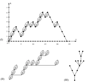
Figure 2: (I) Right excursion of the random walk. Upcrossings are marked by “tree leaves”. (II) The number of upcrossings of the edge(k,k+1)becomes the number of particles in generationkfor the branching process. Shrinking the horizontal lines in (II) into single points gives the tree (III). Traversing the tree (III) in preorder rebuilds the excursion (I).
max{Xn, 0 ≤ n < T0} as illustrated in Figure 2. Moreover, given a tree for a branching process that becomes extinct in finite time, we can reconstruct the right excursion of the random walk. This can be done by making a time diagram of up and down movements of an ant traversing the tree in preorder: the ant starts at the root, always chooses to go up and to the left whenever possible, never returns to an edge that was already crossed in both directions, and finishes the journey at the root (Figure 2, (III)).
The above path-wise correspondence on{T0 <∞} does not depend on the measure associated to
the random walk paths. To consider the set {T0 = ∞} we shall need some of the properties of
this measure. The following simple statement leaves only three major possibilities for a long term behavior of an ERW path.
Lemma 5. Letω∈ΩM. Then P0,ω-a.s.
lim inf
n→∞ Xn, lim supn→∞ Xn∈ {−∞,
+∞}.
Proof. Letz ∈Z. If the ERW visits z infinitely many times then it also visitsz+1 infinitely many
times due to the second Borel Cantelli lemma, the strong Markov property, and the assumption
ω(z,i) = 1/2 for i > M. This implies P0,ω-a.s. lim supnXn ∈/ Z. Similarly, P0,ω-a.s. lim infnXn ∈/ Z.
that the walk starts at 1. Then the probability that T0 <∞is equal to one and the corresponding measure on trees will be the one for a standard Galton-Watson process with the Geom(1/2) offspring distribution starting from a single particle. More precisely, setU0:=1 and let
Uk:=#{n≥0|n<T0, Xn=k, Xn+1=k+1}, k≥1, (9)
be the number of upcrossings of the edge(k,k+1)by the walk before it hits 0. Then(Uk)k≥0has the
same distribution as the Galton-Watson process with Geom(1/2) offspring distribution. Therefore,
(Uk)k≥0 can also be generated as follows: start with one particle: U0=1. To generate the(k+1) -st generation from thek-th generation (assuming that the process has not yet died out), the first particle of generationk tosses a fair coin repeatedly and produces one offspring if the coin comes up "heads". It stops the reproduction once the coin comes up "tails". Then the second particle in generationkfollows the same procedure independently, then the third one, and so on. Consequently,
Uk+1=ξ(k+1)1 +. . .+ξ(k+1)Uk ,
whereξ(j)i ,i,j≥1 are independent with distribution Geom(1/2) .
To construct a branching process corresponding to an ERW with M cookies per site one can use exactly the same procedure except that for the firstM coin tosses in thek-th generation the particles should use coins with biases "prescribed" by the cookies located at sitek. Since every particle tosses a coin at least once, at most the first M particles in each generation will have a chance to use biased coins. All the remaining particles will toss fair coins only. This can be viewed as a branching process with migration in the following natural way. Before the reproduction starts, the firstUk∧M particles emigrate, taking with them allM biased coins and an infinite supply of fair coins. In exile they reproduce according to the procedure described above. Denote the total number of offspring produced by these particles byη(k+1)U
k∧M. Meanwhile, the remaining particles (if any) reproduce using only fair coins. Finally, the offspring of the emigrants re-immigrate. Therefore, the number of particles in the generationk+1 can be written as
Uk+1:=ξ (k+1)
1 +. . .+ξ (k+1) Uk−M+η
(k+1)
Uk∧M, (10)
whereξ(j)i andη(k)ℓ (i,j,k≥1, 0≤ℓ≤M)are independent random variables, each one of the
se-quences(η(k)0 )k≥1, . . . ,(η(k)M )k≥1is identically distributed, and eachξ(j)i has distribution Geom(1/2) .
4
Coin-toss construction of the ERW and the related
(
µ,
ν
)
-branching
process
In this section we formalize a coin-toss construction of the ERW and introduce auxiliary processes used in the rest of the paper.
Let (Ω,F) be some measurable space equipped with a family of probability measures Px,ω, x ∈
Z, ω∈ΩM, such that for each choice of x ∈Zandω∈ΩM we have±1-valued random variables
Yi(k), k∈Z, i≥1, which are independent under Px,
ωwith distribution given by
Px,ω[Yi(k)=1] =ω(k,i) and Px,ω[Yi(k)=−1] =1−ω(k,i).
Moreover, we require that there is a random variableX0on(Ω,F,Px,ω)such thatPx,ω[X0= x] =1.
Then an ERW(Xn)n≥0, starting at x ∈Z, in the environmentωcan be realized on the probability
space(Ω,F,Px,ω)recursively by:
Xn+1 := Xn+Y(Xn)
#{i≤n|Xi=Xn}, n≥0. (11)
We shall refer to{Yi(k)=1}as a “success” and to{Yi(k)=−1}as a “failure”. Due to (11) every step to the right or to the left of the random walk corresponds to a success or a failure, respectively.
We now describe various branching processes that appear in the proofs. Namely, we introduce processes (Vk)k≥0, (Wk)k≥0, and (Zk)k≥0. Modifications of the first two processes suitable for left excursions will be defined later when they are needed (we shall keep the same notation though, hoping that this will not lead to confusion). The last process,(Zk)k≥0, will belong to the class of
processes from Section 2.
Form∈Nandk∈Zlet
S0(k):=0, S(k)m :=# of successes in Yi(k)i≥1prior to them-th failure. (12)
Recall from the introduction thatPx[·]denotes the averaged measureE[Px,ω[·]]. By assumption (2) the walk reaches 1 in one step with positiveP0-probability.
We shall be interested in the behavior of the process(Uk)k≥0 defined in (9). At first, we shall relate (Uk)k≥0to(Vk)k≥0 which is recursively defined by
V0:=1, Vk+1:=S (k+1)
Vk , k≥0. (13)
Observe that(Vk)k≥0is a time homogeneous Markov chain, as the sequence of sequences(S(k)m )m≥0,
k≥0, is i.i.d.. Moreover, 0 is an absorbing state for(Vk)k≥0. We claim that underP1,
Uk=Vk for allk≥0 on the event{T0<∞}; (14)
Uk≤Vk for allk≥0 on the event{T0=∞}. (15)
The relation (14) is obvious from the discussion in Section 3 and Figure 2. To show (15) we shall use induction. Recall thatU0=V0=1 and assumeUi ≤Vi for all i≤ k. From Lemma 5 we know
thatXn→ ∞asn→ ∞on{T0=∞}a.s. with respect toP1. Therefore, the last,Uk-th, upcrossing of
less than or equal to the number of successes in the sequence Yi(k+1)i≥1 prior to theUk-th failure. On the other hand, to get the value of Vk+1 one needs to count all successes in this sequence until theVk-th failure. SinceUk≤Vk, we conclude thatUk+1≤Vk+1.
Next we introduce the process(Wk)k≥0 by setting
W0:=0, Wk+1:=SW(k)k∨M, k≥0. (16)
Just as (Vk)k≥0, the process (Wk)k≥0 is a time homogeneous Markov chain on non-negative inte-gers. Moreover, the transition probabilities from i to j of these two processes coincide except for i ∈ {0, 1, . . . ,M −1} and both processes can reach any positive number with positive probability. Therefore, if one of these two processes goes to infinity with positive probability, so does the other:
P1[Vk→ ∞]>0 ⇐⇒ P1[Wk→ ∞]>0. (17)
Finally, we decompose the process(Wk)k≥0 into two components as follows.
Lemma 6. For k ≥ 0let Zk :=Wk+1−S (k)
M . Then(Zk)k≥0 is a (Geom(1/2),ν)-branching process,
whereν is the common distribution ofηk:=S (k)
M −M under P1.
Proof. By definition,Z0=0 and
Zk+1=Wk+2−S (k+1) M
(16) = SW(k+1)
k+1∨M−S (k+1)
M =ξ
(k+1)
1 +· · ·+ξ (k+1) Wk+1−M,
whereξ(k+1)i is defined as the number of successes in Yj(k+1)j≥1 between the(M+i−1)-th and the(M+i)-th failure,i≥1. Therefore, by definition ofZkandηk,
Zk+1=ξ (k+1)
1 +· · ·+ξ (k+1)
Zk+S (k) M −M
=ξ(k+1)1 +· · ·+ξ(k+1)Z
k+ηk.
Sinceω(k,m) =1/2 for m> M, the random variables Ym(k), m> M, k≥0, are independent and uniformly distributed on {−1, 1} under P1. From this we conclude that the ξ(k)i , k,i ≥ 1, have
distribution Geom(1/2) . To show the independence ofξ(j)i andηk (i,j ≥1, k ≥0), as required
by Definition 1, notice thatηk = S(k)M −M depends only on Ym(k), where mchanges from 1 to the number of the trial resulting in theM-th failure inclusively, while eachξ(k)i ,i≥1, counts the number of successes in Ym(k)m≥1 between the(M+i−1)-th and the(M+i)-th failure. Recalling again that Ym(k),m≥1,k≥0, are independent under P1, we get the desired independence.
Having introduced all necessary processes we can now turn to the proofs of our results.
5
Recurrence and transience
In the next lemma we shall characterize ERW which are recurrent from the right in terms of branch-ing processes with migration. At first, we shall introduce a relaxation of condition (1), which is needed for the proof of Theorem 1:
The sequence(ω(k,·))k≥K is i.i.d. underPfor someK∈N. (18)
Under this assumption the sequence indexed byk≥K of sequences(Yi(k))i≥1is i.i.d. with respect to
P0. In particular, the sequence(S (k)
M )k≥K is i.i.d. underP0.
Lemma 7. Replace assumption (1) by (18) and assumption (2) by
E
M
Y
i=1
(1−ω(K,i))
>0. (19)
Denote the common distribution ofηk := S (k)
M −M , k≥K, under P0byν. Then the ERW is recurrent
from the right if and only if the(Geom(1/2),ν)-branching process dies out a.s., i.e. reaches state0at some time k≥1.
Proof. Since we are interested in the first excursion to the right we may assume without loss of
generality that the random walk starts at 1. Then, recalling definition (9), we have {T0 =∞} =P1
{∀k≥1Uk>0}, whereA P1
=Bmeans that the two eventsAandBmay differ by a P1-null-set only.
Indeed, sinceUk counts only upcrossings of the edge(k,k+1)prior toT0, the inclusion⊇is trivial. The reverse relation follows from Lemma 5. This together with (14) and (15) implies that
{T0=∞}=P1{∀k≥0Vk>0}. (20)
As above(Vk)k≥K is a time homogeneous Markov chain since the sequence of sequences(S(k)m )m≥0, k≥K, is i.i.d.. For anymthe transition probability of this Markov chain fromm∈Nto 0 is equal to
P1[Sm(K)=0] =E
m
Y
i=1
(1−ω(K,i))
,
which is strictly positive by (19). Since 0 is absorbing for(Vk)k≥0 we get that{∀k≥0 Vk >0}=P1
{Vk→ ∞}. Consequently, by (20),{T0=∞}P=1Vk→ ∞ . Next we turn to the process(Wk)k≥0and recall relation (17). Thus,
P1[T0=∞] =0 ⇐⇒ P1[Wk→ ∞] =0. (21)
Finally, we decompose the process(Wk)k≥0 as in Lemma 6 by writingWk+1 = Zk+S (k)
M fork≥0,
where(Zk)k≥K is a Markov chain with the transition kernel of a(Geom(1/2),ν)-branching process. Since the sequence (S(k)M )k≥K is i.i.d., this implies that {Wk → ∞}
P1
= {Zk → ∞}. Together with
Lemma 8. Assume again (1) and (2). If the ERW is recurrent from the right then all excursions to the right of 0 are P0-a.s. finite. If the ERW is not recurrent from the right then it will make P0-a.s. only a
finite number of excursions to the right. The corresponding statements hold for recurrence from the left.
Proof. Let the ERW be recurrent from the right. By Definition 2 the first excursion to the right is a.s. finite. By Lemma 7 the corresponding(Geom(1/2),ν)-branching process dies out a.s.. Leti≥1 and assume that all excursions to the right up to the i-th one have been proven to be P0-a.s. finite.
If the ERW starts the (i+1)-st excursion to the right of 0 then it finds itself in an environment which has been modified by the previousiexcursions up to a random levelR≥1, beyond which the environment has not been touched yet. Therefore, conditioning on the event{R=K},K≥1, puts us within the assumptions of Lemma 7: the random walk starts the right excursion from 0 in a random cookie environment which satisfies (18). But the corresponding(Geom(1/2),ν)-branching process is still the same and, thus, dies out a.s.. Therefore, this excursion, which is the(i+1)-st excursion of the walk, is a.s. finite on{R=K}. Since by our induction assumption the events{R=K},K≥1, form a partition of a set of full measure, we obtain the first statement of the lemma.
For the second statement let
D:=inf{n≥1|Xn<X0}
be the first time that the walk backtracks below its starting point. Due to (2), P0[X1 = 1] > 0.
Therefore, since the walk is assumed to be not recurrent from the right,
P0[D=∞]>0. (22)
Denote by Ki the right-most visited site before the end of the i-th excursion and define Ki = ∞
if there is no i-th right excursion or if the i-th excursion to the right covers N. Then the number
of i ≥ 1 such that Ki < Ki+1, is stochastically bounded from above by a geometric distribution
with parameter P0[D=∞]. Indeed, each time the walk reaches a levelKi+1<∞, which it has never visited before, it has probabilityP0[D=∞]never to backtrack again below the level Ki+1,
independently of its past. Therefore,(Ki)i increases only a finite number of times. Hence P0-a.s. R:=sup{Ki |i≥1,Ki<∞}<∞. Now, if the walk did an infinite number of excursions to the right, then,P0-a.s. supnXn=R<∞and lim supnXn≥0, which is impossible due to Lemma 5.
Proposition 9. The ERW is recurrent from the right if and only ifδ≤1. Similarly, it is recurrent from the left if and only ifδ≥ −1.
For the proof we need the next lemma, which relates the parameterδof the ERW and the parameter
θ of the branching process with migration.
Lemma 10. Let ν be the distribution of S(0)M − M under P0. Then θ defined in (7) for the (Geom(1/2),ν)-branching process is equal toδdefined in (3).
Proof of Lemma 10. Forµ = Geom(1/2) the parameter b defined in (A) equals 1. Hence, by (6),
θ=λ=E0[S(0)M −M]. Thus it suffices to show that
E0[S(0)M ]−M=δ. (23)
number of successes among the firstM trials. Therefore, sinceS(0)M is the total number of successes prior to theM-th failure,S(0)M −(M−F)is the number of successes after theM-th trial and before theM-th failure. GivenF, its distribution is negative binomial with parameters M−F andp=1/2, i.e. the(M−F)-fold convolution of Geom(1/2) , and therefore has meanM−F. Thus,
E0[SM(0)−(M−F)] =E0[E0[SM(0)−(M−F)|F]] =E0[M−F].
SubtractingE0[F]from both sides we obtain
E0[S(0)M ]−M=M−2
M
X
i=1
E[1−ω(0,i)] =
M
X
i=1
(2E[ω(0,i)]−1) =δ.
Proof of Proposition 9. Due to Lemma 7 the walk is recurrent from the right iff the(Geom(1/2),ν) -branching process dies out a.s., where ν is the distribution of S(0)M −M. By the first statement of Corollary 4 this is the case iffθ ≤1. The first claim of the proposition follows now from Lemma 10. The second one follows by symmetry.
Proof of Theorem 1. If δ > 1 then by Proposition 9 the walk is not recurrent from the right but recurrent from the left. If the walk returned infinitely often to 0 then it would also make an infinite number of excursions to the right which is impossible due to Lemma 8. Hence the ERW visits 0 only finitely often. Since any left excursion is finite due to Lemma 8 the last excursion is to the right and is infinite. Consequently,P0-a.s. lim infnXn≥0, and therefore, due to Lemma 5,Xn→ ∞. Similarly,
δ <−1 impliesP0-a.s.Xn→ ∞.
In the remaining caseδ∈[−1, 1]all excursions from 0 are finite due to Proposition 9. Hence, 0 is visited infinitely many times.
Remark 2. The equivalence (20) also holds correspondingly for one-dimensional random walks
(Xn)n≥0 in i.i.d. random environments (RWRE) and branching processes(Vk)k≥0 in random
envi-ronments, i.e. whose offspring distribution is geometric with a random parameter. This way the recurrence theorem due to Solomon[So75, Th. (1.7)] for RWRE can be deduced from results by Athreya and Karlin, see[AN72, Chapter VI.5, Corollary 1 and Theorem 3].
6
A renewal structure for transient ERW
A powerful tool for the study of random walks in random environments (RWRE) is the so-called renewal or regeneration structure. It is already present in [KKS75], [Ke77]and was first used for multi-dimensional RWRE in[SZ99]. It has been mentioned in [Zer05, p. 114, Remark 3]that this renewal structure can be straightforwardly adapted to the setting of directionally transient ERW in i.i.d. environments in order to give a law of large numbers. The proofs of positivity of speed and of a central limit theorem for once-excited random walks in dimension d≥2 in[BR07]were also phrased in terms of this renewal structure. We shall do the same for the present model.
Xτ
1
Xτ2
τ1 τ2 n
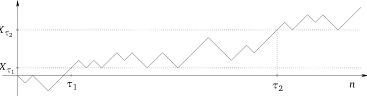
Figure 3: A random walk path with two renewals.
from the right, which implies, as we already mentioned, see (22), thatP0[D=∞]>0. Hence there areP0-a.s. infinitely many random timesn, so-calledrenewalorregeneration times, with the defining property thatXm<Xnfor all 0≤m<nandXm≥Xnfor allm>n. Call the increasing enumeration
of these times(τk)k≥1, see also Figure 3. Then the sequence(Xτ1,τ1),(Xτk+1−Xτk,τk+1−τk) (k≥1)
of random vectors is independent underP0. Furthermore, the random vectors(Xτ
k+1−Xτk,τk+1−
τk), k ≥ 1, have the same distribution under P0. For multidimensional RWRE and once-excited
random walk the corresponding statement is [SZ99, Corollary 1.5] and [BR07, Proposition 3], respectively. It follows from the renewal theorem, see e.g.[Zei04, Lemma 3.2.5], that
E0[Xτ2−Xτ1] =P0[D=∞]−1<∞. (24)
Moreover, the ordinary strong law of large numbers implies that
lim
n→∞ Xn
n = E0[Xτ
2−Xτ1]
E0[τ2−τ1]
=:v P0-a.s., (25)
see[SZ99, Proposition 2.1]and[Zei04, Theorem 3.2.2]for RWRE and also[BR07, Theorem 2]for once-ERW. Therefore,
v>0 if and only if E0[τ2−τ1]<∞. (26)
If, moreover,
E0[(τ2−τ1)2]<∞ (27)
then the result claimed in Theorem 3 holds with
σ2:=
E0hXτ
2−Xτ1−v(τ2−τ1)
2i
E0[τ2−τ1]
>0 (28)
see[Sz00, Theorem 4.1]for RWRE and[BR07, Theorem 3 and Remark 1]for once-ERW.
Thus, in order to prove Theorems 2 and 3 we need to control the first and the second moment, respectively, ofτ2−τ1. We start by introducing fork≥0 the number
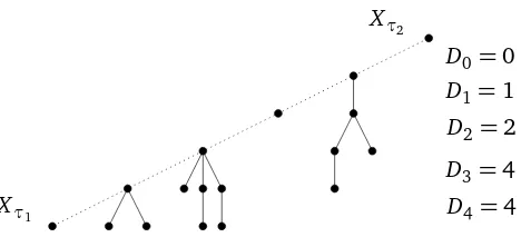
Dk:=#¦n|τ1<n< τ2, Xn=Xτ2−k, Xn+1=Xτ2−k−1
©
(29)
of downcrossings of the edge(Xτ2−k,Xτ2−k−1)between the timesτ1andτ2.
Lemma 11. Assume that the ERW is transient to the right and let p ≥1. Then the p-th moment of
Xτ1
Xτ
2
D0=0
D1=1
D2=2
D3=4
D4=4
Figure 4: For the path in Figure 3 the process(Dk)k≥0 is realized as (0,1,2,4,4,0,0,. . . ). The solid lines represent downcrossings. The thick dots on the dashed line correspond to the single immigrant in definition (32).
Proof. The number of upcrossings betweenτ1 andτ2 isXτ2−Xτ1+
P
k≥1Dk, sinceXτ1 <Xτ2and
since each downcrossing needs to be balanced by an upcrossing. Each step is either an upcrossing or a downcrossing, therefore,
τ2−τ1=Xτ2−Xτ1+2X
k≥1
Dk. (30)
For everyk∈ {Xτ1+1, . . . ,Xτ2−1}there is a downcrossing of the edge(k,k−1), otherwisekwould be another point of renewal. Hence,Xτ
2−Xτ1≤1+
P
k≥1Dkand, by (30),
2X
k≥1
Dk≤τ2−τ1≤1+3
X
k≥1
Dk.
This implies the claim.
To interpret(Dk)k≥0 as a branching process (see Figure 4) we define form∈Nandk∈Z
F0(k):=0, Fm(k):=# of failures in Yi(k)i≥1 prior to them-th success. (31)
(Compare this to the definition ofSm(k)in (12).) Let
V0:=0, Vk+1 := FV(k)
k+1, k≥0; (32)
e
Vk:=Vk1{k<N(V)}, where N(V):=inf{k≥1|Vk=0}. (33)
Lemma 12. Assume that the ERW is transient to the right. Then(Dk)k≥0 and(Vek)k≥0 have the same distribution under P0.
Proof. Fix an integerK ≥1. For brevity, we set ~D:= (D1, . . . ,DK)and~V := (Ve1, . . . ,VeK). It suffices
to show that
P0
~
D=~i=P0
~
V =~i (34)
for all~i ∈NK
0. Since both processes start from 0 and also stay at 0 once they have returned to
0 for the first time, it is enough to consider vectors~iwhose entries are strictly positive except for maybe the last one. And, since the process (Dk)k≥0 eventually does reach 0 P0-a.s., namely at
k=Xτ2−Xτ1<∞, it suffices to consider only~iwhose last entry is 0. Thus, let~i= (i1, . . . ,iK)∈NK
0
withi1, . . . ,iK−1≥1 andiK =0. At first, we shall show that
where, form,k≥0,
D(m)k := #{n<Tm|Xn=m−k, Xn+1=m−k−1} and (36)
~
D(m) := (D(m)1 , . . . ,D(m)K ).
We start from the partition equation
P0
may start the summation in (37) fromm=K. Moreover, comparing the definitions (29) and (36), we see that{~D=~i, τ2=Tm}={~D(m)=~i, τ2=Tm}, using that not only on the left but also on the
Tm and if exactly one of the numbers D (m)
By the strong Markov property applied to the stopping time Tm and by independence in the envi-ronment this equals
Applying the strong Markov property once more, this time toTm−K, and using the i.i.d. structure of the environment, we get that the above is equal to
X
This proves (35). Now we need to show that
P0
is Markov, just as the process (Vek)0≤k≤K. Both processes get absorbed after the first return to 0. Then (39) will follow if we show that they have the same transition probabilities and thatD(K)1 has the same distribution asVe1. Let m≥1 and 1≤k≤K−1 orm=k=0. Notice that if the number
Dk(K)of downcrossings of the edge(K−k,K−k−1)prior toTK ismthen the number of upcrossings
of the same edge prior to TK equalsm+1. Therefore, the number D(Kk+1) of downcrossings of the
edge(K−k−1,K−k−2)prior to TK is equal to the number of failures in Yi(K−k−1)i≥1 before
the(m+1)-st success, which is Fm+1(K−k−1). On the other hand, if Vek = mthen, by (32) and (33),
e
Vk+1=F (k)
m+1. But for alli,j≥0 random variablesF (i)
m+1andF
(j)
m+1 have the same distribution.
7
Law of large numbers and ballisticity
While (25) gives the law of large numbers in the transient case the renewal structure does not say anything about the recurrent case. The following general result covers both the transient and the recurrent case.
Proposition 13. There is a deterministic v∈[−1, 1]such that P0-a.s. Xn/n→v for n→ ∞.
Proof. It can be shown exactly like in the proof of[Zer05, Theorem 13]that if supn≥0Xn =∞a.s. then
lim sup
n→∞ Xn
n ≤
1
u+ a.s., where (40)
u+ := X j≥1
P0[Tj+1−Tj≥ j]∈[1,∞], and
lim inf
n→∞ Xn
n ≥
1 u+
a.s. ifu+<∞ (41)
see the last line on p. 113 and the first line on p. 114 of [Zer05]. Similarly, by symmetry, if infn≥0Xn=−∞a.s. then
lim inf
n→∞ Xn
n ≥
−1
u− a.s., where (42)
u− := X j≥1
P0[T−j−1−T−j≥ j]∈[1,∞], and
lim sup
n→∞ Xn
n ≤
−1
u− a.s. ifu−<∞. (43)
Now due to Theorem 1 there are only three cases: Either the walk is transient to the right or it is transient to the left or it is recurrent. Consider the case of transience to the right. Ifu+ <∞then
limnXn/n=1/u+follows directly from (40) and (41). Ifu+=∞then limnXn/n=0 follows from (40) and infnXn>−∞. Transience to the left is treated analogously. In the case of recurrence we
Lemma 14. Let(Zk)k≥0 be a(Geom(1/2),ν)-branching process, whereν is the distribution ofηk:=
FM(k)−M+1, and recall definitions (8), (32) and (33). Then
E0[Ve]<∞ ⇐⇒E0[eZ]<∞, where Ve:=
X
k≥0
e
Vk and Ze:=
X
k≥0
e
Zk. (44)
Proof. As an intermediate step we first consider the auxiliary Markov chain(Wk)k≥0defined by
W0:=0, Wk+1:=F(W(k)
k+1)∨M. (45)
This is a branching process with migration in the following sense: At each step, it exhibits two types of behavior: 1) ifWk≥M−1 then one particle immigrates and then allWk+1 particles reproduce; 2) ifWk<M−1 thenM−Wkparticles immigrate and then allM particles reproduce.
We shall first establish the equivalence
E0[Ve]<∞ ⇐⇒E0[Wf]<∞. (46)
where, as usual,
N(W):=inf{k≥1|Wk=0}, Wfk:=Wk1{k<N(W)}, and Wf:=
X
k≥0
f
Wk. (47)
Comparing definitions (32) and (45) we see thatVek≤Wfkfor allk, which yields the implication⇐
in (46). For the reverse implication, assume that E0[Ve]is finite. Since N(V)≤ Ve+1 this implies that(Vk)k≥0 is positive recurrent. The following lemma, whose proof is postponed, will help us to compare(Vk)k≥0 and(Wk)k≥0.
Lemma 15. Let K be the transition matrix of a positive recurrent Markov chain with state space N0
and invariant distributionπ. Assume also that all entries of K are strictly positive. Fix a state j ∈N0
and a finite set J⊂N0\ {j}. Modify a finite number of rows of K by setting
K(i,·):=
(
K(i,·), if i6∈J; K(j,·), if i∈J.
Then a Markov chain with the transition matrix K is also positive recurrent and its unique invariant probability distributionπsatisfiesπ(n)≤c6π(n)for all n∈N0.
If we let K be the transition matrix of the Markov chain (Vk)k≥0 and set j = M −1 and J =
{0, 1, . . . ,M−2} then K defined in Lemma 15 is the transition matrix of (Wk)k≥0. Moreover, all entries of this K are strictly positive due to (2). Consequently, we may apply Lemma 15 and get that(Wk)k≥0 is positive recurrent and its invariant probability distributionπis bounded above by a
multiplec6πof the invariant probability distributionπof(Vk)k≥0. By Theorem 5.4.3 of[Du05],π
andπcan be represented asπ=ρ/E0[N(V)]andπ=ρ/E0[N(W)], where fors∈N0,
ρ(s):=E0
N(V) −1
X
k=0
1{Vk=s}
and ρ(s):=E0
N(W) −1
X
k=0
1{Wk=s}
Therefore, alsoρ≤c7ρ. However,
The proof of Lemma 16 is almost identical to the one of Lemma 6 and, thus, is omitted.
Since FM(k)≥0, we immediately obtain Zek′ ≤Wfk+1, where Zek′ is defined by replacingW in (47) by Z′. By Lemma 16,(eZk)k and(eZk′)k have the same distribution. ThereforeE0[Ze] =E0[Ze′]≤E0[Wf],
which yields the implication⇒in (49). For the opposite direction assume that E0[Ze]<∞. Then, as in the proof of (46), (Zk′)k≥0 is positive recurrent and, by the equivalent of (48), its invariant
distribution, sayπ′, has a finite mean. Since Z′
k and F
(k)
M are independent, it follows from Lemma
16 that the convolution ofπ′and the distribution of FM(k)is invariant for(Wk)k≥0. This convolution has a finite mean as well, which implies, as in (48), thatE0[Wf]is finite as well. This concludes the proof of (49). The statement of the lemma now follows from (46) and (49).
Proof of Lemma 15. It suffices to consider the case in whichJ has only one element, i.e. J={i}for somei6= j. The full statement then follows by induction, changing one row at a time. Let(ζk)k≥0
and(ζk)k≥0be Markov chains with transition matricesKandK, respectively. Their initial point will
be denoted by a subscript ofPandE. Since all the entries ofKare strictly positive,Kis irreducible. It is recurrent, since its stateiis recurrent. Indeed,Pi[∃k≥1 :ζk=i] =Pj[∃k≥1 :ζk=i]because
On the other hand, for alls∈N0,
The following lemma is the counterpart of Lemma 10.
Lemma 17. Let ν be the distribution of FM(0)− M +1 under P0. Then θ defined in (7) for the
Proof of Theorem 2. The first statement of the theorem, the existence of the velocityv, is just Propo-sition 13, or (25) in the transient case. Ifδ∈[−1, 1]then the walk is recurrent by Theorem 1 and thereforev=0.
Now let|δ|>1. Without loss of generality we may assumeδ >1. Then the walk is transient to the right by Theorem 1. By (26),v>0 iffE0[τ2−τ1]<∞. By Lemma 11 withp=1 this is the case iff
E0[Wf2]. We shall prove that the latter is finite. By Minkowski’s inequality we have
M defines a(Geom(1/2),ν)-branching process, where
Applying Hölder’s inequality with 1/α+1/α′=1,α >1, we obtain
We are going to show that
(i) for everyǫ∈(0,δ−4)there is a constant c8(ǫ,δ)such that
Let us assume (i) and (ii) for the moment and see that both series in the right hand side of (51) are finite. Chooseα′∈(1,δ/4)so thatα=α′/(α′−1)is an integer and letǫ= (δ−4α′)/2. Then by (i) and (ii) for allk≥1,
E0Zk2−α11/(2α) P0[N(W)>k]1/(2α′)≤c10(α′,δ)k1−(δ−ǫ)/(2α′)=c10k−δ/(4α′).
Sinceδ/(4α′)>1, the first series in the right hand side of (51) converges. It is obvious now that for the same choice of α′ and ǫ the second series in the right hand side of (51) also converges. Therefore we only need to prove (i) and (ii).
Proof of (i).Observe thatWkis zero if and only if bothZk−1andFM(k−1)are equal to zero. SetN0:=0 and consider the timesNi :=inf{k>Ni−1|Zk=0}, i∈N, when the process(Zk)k≥1 dies out. Due
to Lemma 17 andδ >4 the parameterθ for the process(Zk)k≥0 satisfies
θ=1−δ <−3. (52)
In particular, Corollary 4 implies that the process(Zk)k≥0is positive recurrent. Therefore, allNi,i∈
N, are a.s. finite and(Ni−Ni
It is then straightforward to check that eachF(Ni)
M is independent fromFNi,i∈N, and F
M =0 . Thenc has the geometric distribution onN with parameter
From part (iv) of Theorem A and (52) we know that P0[N1 > k] ∼ c4k−δ. Therefore, and since
γ < δby assumption,P0[N1γ >k]is summable ink. Consequently, E0
N1γ=c12(ǫ,δ)<∞. This
implies (i).
Proof of (ii).The proof can be easily done by induction inℓ. The statement is trivial forℓ=0. (Here 00=1.) Assume now ℓ≥1 and that for each j ∈ {0, 1, 2, . . . ,ℓ−1}there is a constantc9(j)such
Observe that the expectation in (54) is bounded by a constantc13(ℓ). To control the series in (55)
we use the following lemma, whose proof is postponed until after the end of the present proof.
Lemma 19. Let(ξi)i∈N be non-negative i.i.d. random variables such that E[ξ1] =1and E
Applying this lemma to the series in (55) we obtain
E0Zk+1ℓ ≤ c13+X (ii) and finishes the proof of Lemma 18.
Proof of Lemma 19. By expanding and using independence,
SinceE[ξ1] =1 the summand form=ℓis equal ton!/(n−ℓ)!≤nℓ. For the other terms we estimate
the factor mnfrom above bynmand define the constant
c14:= max
Proof of Theorem 3. Let|δ|>4. By symmetry we may assume without loss of generality thatδ >4. Then, by Lemma 18, E0[(
9
Further remarks, a multi-dimensional example, and open questions
Remark 3(Permuting cookies). Note that permuting cookies within the cookie piles, i.e. replacing
(ω(·,i))i≥1 by ω(·,π(i))i≥1, where π : N → N is a permutation, does not change δ, defined in
(3). Therefore, permuting cookies does not change the classification of the walk as described in Theorems 1 and 2. This fact can also be seen as follows without using the results in Theorem A from the literature.
At first, observe that we may assume without loss of generality thatπis a finite permutation, since all cookies in a cookie pile except for a finite number are placebo cookies. We may even assume that all i>M are fixed points forπ. Indeed, otherwise just replace the original M with max{π(i)|i≤M}. To argue, for example, that permuting cookies does not turn a walk which is recurrent from the right into one which is not recurrent from the right or vice versa, recall the definition ofS(k)M in (12) and ofηk in Lemma 7 and denote byσ the M-th failure in the permuted sequenceYπ(k)(i). This shows that applyingπ does not change the distributionν ofηk. Therefore, recurrence to the right, as characterized in Lemma 7, is invariant
under permutations. Since the proof of Lemma 7 did not use any results from Section 2, this proof is self-contained.
Similarly, one can show that the positivity of speed is invariant under permutations. Indeed, in the proof of Theorem 2 we have shown thatv >0 iff E0[Pk≥0eZk]<∞. By the above argument, the distribution of(Zek)k≥0remains unchanged under permutations.
Remark 4(Higher dimensions). Multi-dimensional ERW with cookies that induce a bias with a non-negative projection in some fixed direction were considered in[BW03], [Ko03], [Ko05], [Zer06],