07350015%2E2013%2E844155

(1)

Full Terms & Conditions of access and use can be found at

http://www.tandfonline.com/action/journalInformation?journalCode=ubes20 Download by: [Universitas Maritim Raja Ali Haji], [UNIVERSITAS MARITIM RAJA ALI HAJI

TANJUNGPINANG, KEPULAUAN RIAU] Date: 11 January 2016, At: 20:33

Journal of Business & Economic Statistics

ISSN: 0735-0015 (Print) 1537-2707 (Online) Journal homepage: http://www.tandfonline.com/loi/ubes20

Nowcasting GDP in Real Time: A Density

Combination Approach

Knut Are Aastveit, Karsten R. Gerdrup, Anne Sofie Jore & Leif Anders

Thorsrud

To cite this article: Knut Are Aastveit, Karsten R. Gerdrup, Anne Sofie Jore & Leif Anders Thorsrud (2014) Nowcasting GDP in Real Time: A Density Combination Approach, Journal of Business & Economic Statistics, 32:1, 48-68, DOI: 10.1080/07350015.2013.844155

To link to this article: http://dx.doi.org/10.1080/07350015.2013.844155

View supplementary material

Accepted author version posted online: 25 Sep 2013.

Submit your article to this journal

Article views: 493

View related articles

(2)

Nowcasting GDP in Real Time: A Density

Combination Approach

Knut Are AASTVEIT, Karsten R. GERDRUP, and Anne Sofie JORE

Monetary Policy Department, Norges Bank, NO-0107 Oslo, Norway

(Knut-Are.Aastveit@norges-bank.no;Karsten.Gerdrup@norges-bank.no;Anne-Sofie.Jore@norges-bank.no)

Leif Anders THORSRUD

Department of Economics, BI Norwegian Business School and Norges Bank, Oslo, Norway (Leif.A.Thorsrud@bi.no)

In this article, we use U.S. real-time data to produce combined density nowcasts of quarterly Gross Domestic Product (GDP) growth, using a system of three commonly used model classes. We update the density nowcast for every new data release throughout the quarter, and highlight the importance of new information for nowcasting. Our results show that the logarithmic score of the predictive densities for U.S. GDP growth increase almost monotonically, as new information arrives during the quarter. While the ranking of the model classes changes during the quarter, the combined density nowcasts always perform well relative to the model classes in terms of both logarithmic scores and calibration tests. The density combination approach is superior to a simple model selection strategy and also performs better in terms of point forecast evaluation than standard point forecast combinations.

KEY WORDS: Forecast densities; Forecast evaluation; Monetary policy; Real-time data.

1. INTRODUCTION

Economic decision making in real time is based on assess-ments of the recent past and current economic conditions, under a high degree of uncertainty. Many key statistics are released with a long delay, are subsequently revised, and are available at different frequencies. As a consequence, there has been sub-stantial interest in developing a framework for forecasting the present and recent past, that is, nowcasting (see Banbura, Gian-none, and Reichlin2011for a survey of nowcasting).

Until recently, the academic literature on nowcasting has fo-cused on developing single models that increase forecast accu-racy in terms of point nowcast (see, among others, Evans2005; Giannone, Reichlin, and Small 2008; Kuzin, Marcellino, and Schumacher 2011). This differs in two important ways from economic decision making in practice.

First, as the data-generating process is unknown and likely to change over time, decision makers are often given several different models that may produce different forecasts. This nat-urally leads to the question of what forecast or combination of forecasts should be used. The idea of combining forecasts of different models was first introduced by Bates and Granger (1969). Timmermann (2006) provided an extensive survey of different combination methods.

Second, if the decision maker’s loss function is not quadratic, it no longer suffices to focus solely on first moments of possi-ble outcomes (point forecasts). To ensure appropriate decision making, the decision maker should be given suitable characteri-zations of forecast uncertainty. Density forecasts provide an esti-mate of the probability distribution of forecasts. Gneiting (2011) discussed in detail the difference between point forecasting and density forecasting, while Mitchell and Hall (2005) and Hall and Mitchell (2007) provided a justification for density combination. In this article, we combine density nowcasts of U.S. Gross Domestic Product (GDP) growth from three different model

classes: bridge equation models, factor models (FMs), and mixed-frequency vector autoregressive (MF-VAR) models, all widely used for short-term macroeconomic forecasting. More precisely, we extend the use of bridge equation models, as in Baffigi, Golinelli, and Parigi (2004) and Angelini et al. (2011), FMs, as in Giannone, Reichlin, and Small (2008), and MF-VAR models, as in Kuzin, Marcellino, and Schumacher (2011), to produce density nowcasts for a wide range of different model specifications within each model class. Our recursive nowcast-ing exercise is applied to U.S. real-time data. We update the density nowcasts for every new data release during a quarter and highlight the importance of new data releases for the eval-uation period 1990Q2–2010Q3.

The density nowcasts are combined in a two-step procedure. In the first step, nowcasts from all individual models within a model class are combined, using their logarithmic scores (log score) to compute their weights (see, among others, Jore, Mitchell, and Vahey2010). This yields a combined density now-cast for each of the three model classes. In a second step, these three predictive densities are combined into a single density nowcast, again using log score weights. The advantages of this approach are that it explicitly accounts for uncertainty of model specification and instabilities within each model class, and that it implicitly gives a priori equal weight to each model class. We evaluate our density nowcasts both in terms of scoring rules and the probability integral transforms, to check whether predictive densities are accurate and well calibrated.

Our novel approach of combining density nowcasts from dif-ferent model classes extends the findings of earlier nowcasting and forecast combination literature in several ways.

January 2014, Vol. 32, No. 1 DOI:10.1080/07350015.2013.844155

48

(3)

Aastveit et al.: Nowcasting GDP in Real Time: A Density Combination Approach 49

First, we show that the log scores of the final combined pre-dictive densities, as well as the prepre-dictive densities of the three model classes, increase almost monotonically as new informa-tion arrives during the quarter. The final combined densities seem well calibrated. Our exercise is close to that of Gian-none, Reichlin, and Small (2008), who apply a dynamic FM, showing that the root mean square forecasting error decreases monotonically with each data release. The importance of using nonsynchronous data releases (the jagged edge problem) for point nowcasting has also been highlighted by Evans (2005) and Banbura and R¨unstler (2011).

Second, we show that while the ranking of the model classes changes during the quarter as new data are released, the final combined density nowcast always performs well relative to the model classes. Furthermore, our combined density nowcasts outperform nowcasts based on a simple selection strategy. This result extends the findings reported in, for example, R¨unstler et al. (2009), who studied point forecasts and model selection strategies.

Third, we find that in our application, the density combination framework also performs better than standard point forecast combination methods in terms of point forecast evaluation.

The two articles most closely related to ours are Kuzin, Mar-cellino, and Schumacher (2013) and Mazzi, Mitchell, and Mon-tana (in press). Kuzin, Marcellino, and Schumacher (in press) studied pooling versus model selection for nowcasting, finding that pooling provides more stable and, in most cases, better point nowcasts than model selection. Our analysis confirms these re-sults, when evaluating density nowcasts for GDP growth using 120 variables, grouped into 15 data block releases, during each month of a quarter. Mazzi, Mitchell, and Montana (in press) combined a small set of leading indicator models to construct density nowcasts for Euro-area GDP growth. They focused par-ticularly on the ability to probabilistically anticipate the 2008– 2009 Euro-area recession. Our approach differs from theirs, as we combine a wide set of models and study in detail the impor-tance of monthly data releases over a 20-year period.

Finally, our study also has similarities with, and supplement the findings of, for example, Bache et al. (2011) and Geweke and Amisano (2011), all of whom combine density forecasts from different types of models, but do not study nowcasting.

Our results are robust to various robustness checks. Comput-ing model weights and evaluatComput-ing final densities usComput-ing different real-time data vintages do not alter the qualitative results. While the nowcasting performance of different model classes may vary according to benchmark vintage, the combined density nowcast always performs well. Changing the weighting scheme by us-ing equal weights and/or combinus-ing forecasts from all models in one step has no effect on our conclusions: performance improves almost monotonically throughout the quarter as new informa-tion becomes available, and the combinainforma-tion approach is still superior to the selection strategy.

The remainder of the article is organized as follows. In the next section, we describe the real-time dataset. In the third sec-tion, we describe the modeling framework and discuss the ratio-nale for combining densities of different model classes, while in the fourth section we describe the recursive forecasting ex-ercise. In the fifth section, we present the results of our out-of-sample nowcasting experiment. Finally, we conclude in the sixth section.

2. DATA

Our aim is to evaluate the current quarter density nowcast of the quarterly growth rate of GDP. Accordingly, in our forecast-ing experiment, we consider 120 monthly leadforecast-ing indicators to nowcast quarterly growth in U.S. GDP.

The monthly data are mainly collected from the ALFRED (ArchivaL Federal Reserve Economic Data) database main-tained by the Federal Reserve Bank of St. Louis. This database consists of collections of real-time vintages of data for each variable. Vintages vary across time as either new data are re-leased or existing data are revised by the relevant statistical agency. Using data from this database ensures that we are using only data that were available on the date of the forecast ori-gin. In addition, several real-time data series are collected from the Federal Reserve Bank of Philadelphia’s Real-Time Data Set for Macroeconomists. Only quarterly vintages are available for these series, where each vintage reflects the information avail-able around the middle of the respective quarter. Croushore and Stark (2001) provided a description of the database.

Some of the series we use, for example, financial market data, are not revised. Other variables, such as consumer prices and most survey data, only undergo revisions due to changes in seasonal factors. When real-time vintage data are not avail-able for these variavail-ables, we use the last availavail-able data vintage as their real-time observations. These data series are collected from Reuters EcoWin. Series such as equity prices, dividend yields, currency rates, interest rates, and commodity prices are constructed as monthly averages of daily observations. Finally, for some series, such as disaggregated measures of industrial production, real-time vintage data exist only for parts of the evaluation period. For such variables, we use the first available real-time vintage and truncate these series backward recursively. A more detailed description of the data series and the availability of real-time vintages are given in AppendixD.

The full forecast evaluation period runs from 1990Q2 to 2010Q3. We use monthly real-time data with quarterly vintages from 1990Q3 to 2010Q4, that is, we do not take account of data revisions in the monthly variables within a quarter. The quar-terly vintages reflect information available just before the first release of the GDP estimate. The starting point of the estima-tion period is 1982M1. A key issue in this exercise is the choice of a benchmark for the “actual” measure of GDP. Stark and Croushore (2002) discussed three alternative benchmark data vintages: the most recent data vintage, the last vintage before a structural revision (called a benchmark vintage), and finally the estimate that is released a fixed period of time after the first release. We follow Romer and Romer (2000) in using the second available estimate of GDP as the actual measure. We have also computed results using the fifth release and the last available vintage of GDP, finding that qualitatively there are no major changes (see Section5.4). The nowcasting exercise is described in more detail in Section4.

3. FORECAST FRAMEWORK

Combining density forecasts is a rather new field of study in economics. The novel aspect of our study is that we combine predictive densities for nowcasting. As we nowcast quarterly U.S. GDP growth on the basis of the flow of information that

(4)

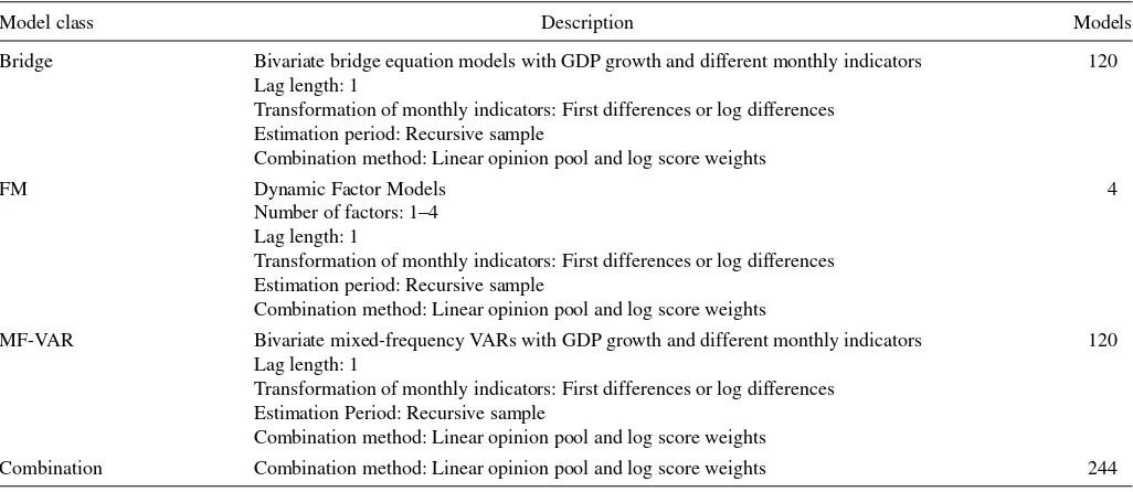
Table 1. A summary of all models and model classes

Model class Description Models

Bridge Bivariate bridge equation models with GDP growth and different monthly indicators 120

Lag length: 1

Transformation of monthly indicators: First differences or log differences Estimation period: Recursive sample

Combination method: Linear opinion pool and log score weights

FM Dynamic Factor Models 4

Number of factors: 1–4 Lag length: 1

Transformation of monthly indicators: First differences or log differences Estimation period: Recursive sample

MF-VAR Bivariate mixed-frequency VARs with GDP growth and different monthly indicators 120

Lag length: 1

Transformation of monthly indicators: First differences or log differences Estimation Period: Recursive sample

Combination Combination method: Linear opinion pool and log score weights 244

NOTE: Each model class is described in more detail in AppendixA. The estimation period begins in 1982M1, for all models.

becomes available during the quarter, the individual models in the forecast framework must accommodate both missing obser-vations and time aggregations from monthly to quarterly fre-quencies. We use a system of three different model classes suit-able to this task: bridge equation models (Bridge), MF-VARs, and FMs. Lately, increased interest has also been given to mixed data sampling (MIDAS) models (see, among others, Clements and Galv˜ao2008,2009; Ghysels and Wright2009; Kuzin, Mar-cellino, and Schumacher2011). We abstract from this type of model in our combination framework, since the scope of models is already fairly exhaustive, and the MIDAS approach has not yet been extended to density forecasting.

For each model class, there is considerable uncertainty re-garding specification, for example, choice of lag length, which variables to include, number of factors, etc. Recent work by Clark and McCracken (2009,2010) shows that VARs may be prone to instabilities. The authors suggest combining forecasts from a wide range of VAR specifications to circumvent these problems. In our application, we include a wide range of speci-fications for each of the three model classes.

In total, we include 244 individual models, distributed un-evenly among the three model classes. Importantly, each indi-vidual model must produce density forecasts. We do this using bootstrapping techniques that account for both parameter and shock uncertainty.Table 1provides a short overview of the dif-ferent specifications within each model class, while AppendixA

summarizes the estimation and simulation procedures. Details about the different model classes can be found in the appendices and in Angelini et al. (2011) (Bridge), Giannone, Reichlin, and Small (2008) (FM), and Kuzin, Marcellino, and Schumacher (2011) (MF-VAR).

We combine the forecasts in two steps (see Garratt, Mitchell, and Vahey 2009; Bache et al. 2011 for a similar procedure). In the first step, nowcasts from all individual models within a model class are combined. This yields one combined predictive density for each model class. In the second step, we combine

density nowcasts from the three model classes to obtain a sin-gle combined density nowcast. An advantage of this approach is that it explicitly accounts for uncertainty about model spec-ification and instabilities within each model class. Hence, our predictive densities for each model class will be more robust to mis-specification and instabilities than if we were to follow the common approach in which only one model from each model class is used. Furthermore, the two-step procedure ensures that, a priori, we put equal weight on each model class. Our approach is close to Aiolfi and Timmermann (2006) in the sense that we combine forecasts in more than one step. They found that fore-casting performance can be improved by first sorting models into clusters based on their past performance, then pooling fore-casts within each cluster, and finally estimating weights for the clusters.

3.1 Combining Predictive Densities

To combine density forecasts, we employ the linear opinion pool:

p(yτ,h)= N

i=1

wi,τ,hg(yτ,h|Ii,τ), τ =τ , . . . , τ , (1)

whereNdenotes the number of models to combine,Ii,τ is the information set used by modeliat timeτto produce the density forecastg(yτ,h|Ii,τ) for variableyat forecasting horizonh.τand τ are the periods over which the individual densities are eval-uated, andwi,τ,hare a set of time-varying nonnegative weights that sum to unity.

CombiningNdensity forecasts according to Equation (1) can potentially produce a combined density forecast with character-istics quite different from those of the individual densities. As Hall and Mitchell (2007) noted, if all the individual densities are normal, but have different mean and variance, the combined density forecast using the linear opinion pool will be mixture

(5)

normal. This distribution can accommodate both skewness and kurtosis and be multimodal (see Kascha and Ravazzolo2010). If the true unknown density is nonnormal, this is an appealing feature. As the combined density is a linear combination of all the individual densities, the variance of the combined density forecast will generally be higher than that of the individual mod-els. The reason for this is that the variance of the combination is a weighted sum of a measure of model uncertainty and disper-sion of (or disagreement about) the point forecast (see Wallis

2005). However, as shown in Gneiting and Ranjan (2013), if the individual densities are correctly calibrated, the higher variance of the combined density may lead to too dispersed densities.

We construct recursive weights based on the fit of the indi-vidual predictive densities. To measure the density fit for each model through the evaluation period, we use the logarithmic score (see Amisano and Giacomini 2007; Hall and Mitchell

2007). The log score is the logarithm of a probability density function evaluated at the outturn of the forecast, providing an intuitive measure of density fit. Hoeting et al. (1999) also argued that the log score can be seen as a combined measure of bias and calibration. A weighting scheme based on the log score is appealing as it gives high weights to predictive densities that assign high probabilities to the realized value.

Following Jore, Mitchell, and Vahey (2010), the recursive weights,wi,τ,h, for theh-step ahead densities can be expressed as ability density function evaluated at the outturn, yτ,h, of the density forecast,g(yτ,h|Ii,τ), andτ −2 toτcomprises the train-ing period used to initialize the weights. The recursive weights are derived based on out-of-sample performance, and they are horizon specific.

Weighting schemes based on the log score have also been ap-plied by Geweke and Amisano (2011), Kascha and Ravazzolo (2010), Bjørnland et al. (2011), Mitchell and Wallis (2011), and Mazzi, Mitchell, and Montana (in press). For point forecast combinations, weighting schemes based on equally weighted combinations and weights derived from the sum of squared forecast errors (SSEs) have been found to work well, both em-pirically and theoretically (see, e.g., Bates and Granger1969; Clemen1989; Stock and Watson2004). Accordingly, we also consider these weighting schemes.

3.2 Evaluating Density Forecasts

We evaluate the (combined) density forecasts by computing the average log score over the evaluation sample, and, follow-ing Diebold, Gunther, and Tay (1998), by testing goodness of fit relative to the ”true,” but unobserved density using the probabil-ity integral transforms (pits). As described above, the (average) log score is an intuitive measure of density fit, while the pits summarize the properties of the densities and may help us judge whether the densities are biased in a particular direction and

whether the width of the densities have been roughly correct on average. More precisely, the pits represent the ex ante in-verse predictive cumulative distributions, evaluated at the ex post actual observations.

We gauge calibration by examining whether the pits are uni-form and identically and (for one-step ahead forecasts) inde-pendently distributed over the interval [0,1]. Several candidate tests exist, but few offer a composite test of both uniformity and independence, as would be appropriate for one-step ahead forecasts.

Thus, we conduct several different tests. We use a test of uniformity of the pits proposed by Berkowitz (2001). The Berkowitz test works with the inverse normal cumulative den-sity function transformation of the pits, which permits testing for normality instead of for uniformity. For one-step ahead fore-casts, the null hypothesis is that the transformed pits are iid

N(0,1). The test statistic isχ2_{, with three degrees of freedom.}

For longer horizons, we do not test for independence, and thus the null hypothesis is that the transformed pits are identically standard normally distributed. The test statistics are then χ2, with two degrees of freedom. Other tests of uniformity em-ployed are the Anderson–Darling (AD) test (see Noceti, Smith, and Hodges2003) and a Pearson chi-squared test, as suggested by Wallis (2003). Note that the latter two tests are more suit-able for small samples. Independence of the pits is tested using Ljung–Box tests, based on autocorrelation coefficients of up to four for one-step ahead forecasts. For forecast horizonh >1, we test for autocorrelation with lags equal to or greater thanhusing a modified Ljung–Box test. See Corradi and Swanson (2006) and Hall and Mitchell (2007) for more elaborate descriptions of the different tests.

Finally, note that passing the various pits tests is necessary, but not sufficient, for a forecast density to be considered the “true” density, conditional on the information set at the time the forecast is made.

4. EMPIRICAL EXERCISE AND ORDERING

OF DATA BLOCKS

We perform a real-time out-of-sample nowcasting exercise for quarterly U.S. GDP growth for the period 1990Q2–2010Q3. The exercise is constructed as follows: for each vintage of GDP values, we estimate all models and compute density nowcasts (for all individual models, model classes, and combinations) for every new data release within the quarter until publication of the first GDP estimate. This occurs approximately 3 weeks after the end of the quarter. By then, the nowcast will have become a backcast for that quarter.

Our dataset consists of 120 monthly variables. Series that have similar release dates and are similar in content are grouped together in blocks. The structure of the unbalancedness changes when a new block is released. In total, we have defined 15 dif-ferent monthly blocks, where the number of variables in each block varies from 30, in “Labor Market,” to only one, in “Ini-tial Claims.” On some dates, more than one block is released. However, our results are robust to alternative orderings of the blocks.

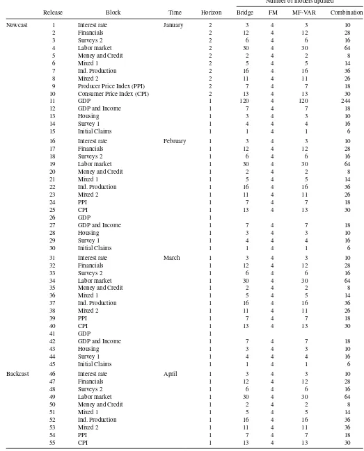
InTable 2, we illustrate the data release calendar and show

how the 15 blocks are released throughout each month and

(6)

Table 2. Structure of data releases and models updated from the start of the quarter until the first estimate of GDP is released

Number of models updated

Release Block Time Horizon Bridge FM MF-VAR Combination

Nowcast 1 Interest rate January 2 3 4 3 10

2 Financials 2 12 4 12 28

3 Surveys 2 2 6 4 6 16

4 Labor market 2 30 4 30 64

5 Money and Credit 2 2 4 2 8

6 Mixed 1 2 5 4 5 14

7 Ind. Production 2 16 4 16 36

8 Mixed 2 2 11 4 11 26

9 Producer Price Index (PPI) 2 7 4 7 18

10 Consumer Price Index (CPI) 2 13 4 13 30

11 GDP 1 120 4 120 244

12 GDP and Income 1 7 4 7 18

13 Housing 1 3 4 3 10

14 Survey 1 1 4 4 4 16

15 Initial Claims 1 1 4 1 6

16 Interest rate February 1 3 4 3 10

17 Financials 1 12 4 12 28

18 Surveys 2 1 6 4 6 16

19 Labor market 1 30 4 30 64

21 Mixed 1 1 5 4 5 14

23 Mixed 2 1 11 4 11 26

24 PPI 1 7 4 7 18

25 CPI 1 13 4 13 30

26 GDP 1

28 Housing 1 3 4 3 10

29 Survey 1 1 4 4 4 16

31 Interest rate March 1 3 4 3 10

32 Financials 1 12 4 12 28

33 Surveys 2 1 6 4 6 16

34 Labor market 1 30 4 30 64

36 Mixed 1 1 5 4 5 14

38 Mixed 2 1 11 4 11 26

39 PPI 1 7 4 7 18

40 CPI 1 13 4 13 30

41 GDP 1

43 Housing 1 3 4 3 10

44 Survey 1 1 4 4 4 16

Backcast 46 Interest rate April 1 3 4 3 10

47 Financials 1 12 4 12 28

48 Surveys 2 1 6 4 6 16

49 Labor market 1 30 4 30 64

51 Mixed 1 1 5 4 5 14

53 Mixed 2 1 11 4 11 36

54 PPI 1 7 4 7 18

55 CPI 1 13 4 13 30

NOTE: The table illustrates a generic quarter of real-time out-of-sample forecasting experiments. Our forecast evaluation period runs from 1990Q2 to 2010Q3, which gives us more than 80 observations to evaluate, for each data release. All models that are updated are reestimated at each point in time throughout the quarter. In total, we reestimate and simulate (bootstrap) the individual models 2000 times for every block in a given quarter.

(7)

Aastv Money & Credit Mixed 1 GDP & Income

Housing Money & Credit Mixed 1 Ind.Production

Mixed 2 PPI CPI GDP & Income

Housing Money & Credit Mixed 1 Money & Credit Mixed 1 GDP & Income

Housing Money & Credit Mixed 1

(8)

0

Financial _Sur

v

Money & Credit

Mixed 1

GDP & Income

Ho

Financial _Sur

v

Money & Credit

Mixed 1

GDP & Income

Ho

Financial _Sur

v

Money & Credit

Mixed 1

GDP & Income

Ho

Financial _Sur

v

Money & Credit

Mixed 1

Financial _Sur

v

Money & Credit

Mixed 1

GDP & Income

Ho

Financial _Sur

v

Money & Credit

Mixed 1

GDP & Income

Ho

Financial _Sur

v

Money & Credit

Mixed 1

GDP & Income

Ho

Financial _Sur

v

Money & Credit

Mixed 1

Financial _Sur

v

Money & Credit

Mixed 1

GDP & Income

Ho

Financial _Sur

v

Money & Credit

Mixed 1

GDP & Income

Ho

Financial _Sur

v

Money & Credit

Mixed 1

GDP & Income

Ho

Financial _Sur

v

Money & Credit

Mixed 1

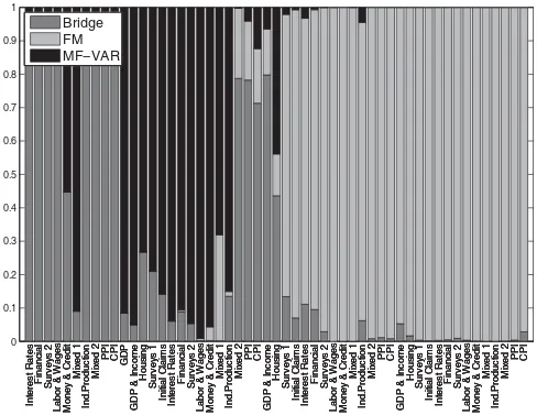
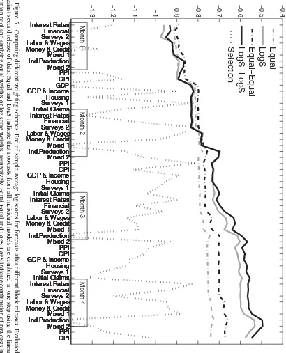
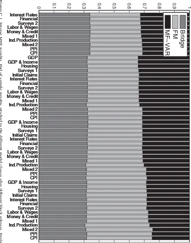
Figure 2. End of sample weights attached to the different model classes after different block releases. Evaluated against second release of data.

quarter is somewhat surprising as these models usually deliver good point nowcasts. This is also the case in our application. However, as discussed in the next section, the densities from the FM class seem to be too narrow at the beginning of the quarter. As the log score strongly penalize realizations in the outer tails of the predictive distribution, the FM class gets a lower average score than the other model classes.

Figure 2shows how the weights attached to each model class

in the combined density nowcast change after each data block release. The figure illustrates the weights at the end of the eval-uation period. As the weights are based on past log score perfor-mance, the same pattern as that observed in the average log score comparison arises. That is, the Bridge and MF-VAR classes have high weight in the early periods of the quarter, while the FM class winds up having nearly all the weight toward the end of the quarter. The reader, however, should not interpret this as attaching all weight to one unique model, as the FM class is in fact a combination of four FMs.

Finally, note that the average log score of the combined den-sity nowcast is almost identical to that of the best performing model class throughout the quarter. This illustrates the main advantage of using forecast combinations.

5.2 Calibration

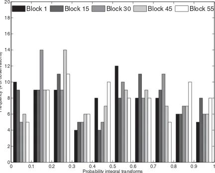
We evaluate the predictive densities relative to the “true,” but unobserved, density, using the pits (seeFigure 3).Table 3

showsp-values for the four different tests described in Section

3.2, applied to the combined forecast at five different points in time. The latter correspond to the start of the first month (Block 1), the end of the first month (Block 15), the end of the second month (Block 30), the end of the third month (Block 45), and the middle of the fourth month (Block 55).p-Values equal to or higher than 0.05 mean that we cannot reject, at the 5% significance level, the hypothesis that the combined predictive density is correctly calibrated.

The combined density nowcast, where the nowcast corre-sponds to a two-step ahead forecast, passes all the tests for Block 1. Turning to the one-step ahead forecast (Block 15– Block 55), the combined density nowcast also seems to be well calibrated. Based on the Berkowitz test, the AD test, and the Pearson chi-squared test, we cannot reject, at a 5% signifi-cance level, the null hypothesis that the combined density is well calibrated. One exception is that the null hypothesis in the Ljung–Box tests (LB1 and LB3) are rejected for Block 55.

(9)

0 0.1 0.2 0.3 0.4 0.5 0.6 0.7 0.8 0.9 1

0 2 4 6 8 10 12 14 16 18 20

Probability integral transforms

Freq

u

ency (# of o

b

ser

v

ations)

Block 1

Block 15

Block 30

Block 45

Block 55

Figure 3. Pits of the combined density forecasts at five points during the quarter. The pits are the ex ante inverse predictive cumulative distributions, evaluated at the ex post actual observations. The pits of predictive densities should have a standard uniform distribution, if the model is correctly specified.

Tables B.1–B.3 in Appendix B report p-values for the calibration tests for nowcasts from each of the three model classes. While density nowcasts from the Bridge and MF-VAR classes seem to be well calibrated, test results for the FM class are a bit more mixed. In particular the null hypothesis in

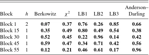
Table 3. Pits tests for evaluating density forecasts for GDP growth

Anderson–

Block h Berkowitz χ2 _LB1 _LB2 _LB3 _Darling

Block 1 2 0.13 0.72 0.94 0.73 0.80 1.03

Block 15 1 0.29 0.13 0.72 0.60 0.58 0.56

Block 30 1 0.70 0.59 0.16 0.83 0.20 0.55

Block 45 1 0.65 0.49 0.07 0.60 0.15 0.61

Block 55 1 0.87 0.85 0.01 0.59 0.03 0.50

NOTE: For Block 15, Block 30, and Block 45, the nowcast is a one-step ahead forecast, while it is a two-step ahead forecast for Block 1. Block 55 is a one-step ahead backcast. All numbers arep-values, except for the Anderson–Darling test. The null hypothesis in the Berkowitz test is that the inverse normal cumulative distribution function transformed pits areidN(0,1), and forh=1 are independent.χ2_{is the Pearson chi-squared test suggested} by Wallis (2003) of uniformity of the pits histogram in eight equiprobable classes. LB1, LB2, and LB3 are Ljung–Box tests of independence of the pits in the first, second, and third power, respectively, at lags greater than or equal to the horizon. Assuming independence of the pits, the Anderson–Darling test statistic for uniformity of the pits has a 5% small-sample (simulated) critical value of 2.5. Numbers in bold indicate that we cannot reject, at the 5% significance level, the null hypothesis that the density is well calibrated.

the Ljung–Box test (LB 1) is rejected for all reported blocks (except Block 1) and the null hypothesis in the Berkowitz test is rejected for Block 1 and Block 15. The latter is consistent with the densities from the FM class being too narrow at the beginning of the quarter.

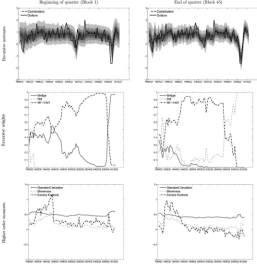
5.3 Properties of the Density Nowcasts

Some properties of the density nowcasts are illustrated in

Figure 4. In the first row, the figure shows recursive real-time

out-of-sample density nowcasts for U.S. GDP growth for the pe-riod 1990Q2–2010Q3. Recursive nowcasts made on the first day of the quarter (Block 1) are shown in the left panel, while recur-sive nowcasts made on the last day of the quarter (Block 45) are shown in the right panel. The two panels illustrate how the pre-cision of the predictive densities improves as more information becomes available.

The second row in the figure shows how the recursive weights change over time. There are large movements in the weights related to the start of the Great Recession, for nowcasts made at Block 1 and Block 45. For nowcasts made at Block 45, there is also a shift in the weights during the expansion of 2006–2007. Finally, as noted in Section3.1, using a linear opinion pool to combine density nowcasts may yield a predictive density that

(10)

Figure 4. Recursive real-time out-of-sample density nowcasts for quarterly U.S. GDP. Results from Block 1 are in the left column, and results from Block 45 are in the right column. The shaded areas for the recursive nowcasts represent 30%, 50%, 70%, and 90% probability bands, respectively.

deviates from normality. The lower row in the figure shows how the behavior of higher-order moments of the combined predictive density evolve over time. The standard deviation is rather stable over time, but increases, in particular for Block 1 nowcasts, during the Great Recession. Interestingly, Carriero, Clark, and Marcellino (2012) found a similar pattern when using a mixed-frequency model with stochastic volatility. There are larger movements in skewness and excess kurtosis over time. For Block 1 and Block 45 nowcasts, there is evidence of positive skewness and positive excess kurtosis in the early parts of the

sample. Also, at the end of the sample, the density nowcasts appear to deviate from normality. The movements in the higher-order moments correspond with changes in the weights attached to the different model classes.

5.4 Robustness

In this section, we perform three robustness checks: first, with respect to alternative weighting schemes; second, with respect

(11)

Aastv Money & Credit Mixed 1 GDP & Income

(12)

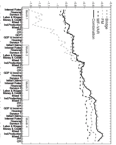
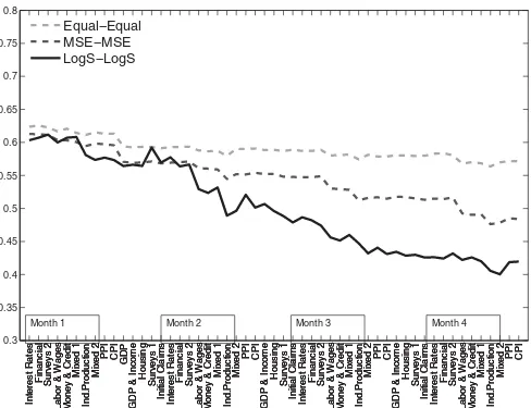
5.4.2 Point Forecasting. We also investigate robustness of our results by evaluating point nowcasting performance. We do this by comparing three different two-step combination strate-gies. First, we use the “LogS-LogS” approach, calculating point nowcasts as the mean of the combined density nowcast. Second, we apply inverse mean squared error (MSE) weights (MSE-MSE) (see, among others, Bjørnland et al.2012for a formula for applying inverse MSE weights), and calculate point nowcasts. Finally, we calculate the point nowcast using the “Equal-Equal” approach. We evaluate the point nowcasts of the three different combination approaches, using the root mean squared predic-tion error (RMSE). The remainder of the experiment is similar to what we have described above.

Figure 6depicts the RMSE for the combined nowcasts, using

the three strategies, after each data block release. The figure displays two key results. First, for all strategies, nowcasting errors steadily decline as more information becomes available throughout the quarter until the first GDP estimate is released. This result accords with the findings of earlier nowcasting exper-iments that used MSE evaluation (see, e.g., Giannone, Reichlin, and Small2008).

Second, the density combination approach (“LogS-LogS”) performs better, in terms of RMSE, than the strategy of applying inverse MSE weights. ComparingFigure 2in the main text and

Figure C.1 in Appendix C, we see that as new information

arrives during the quarter, the log score weights adapt faster than the inverse MSE weights. This does not need to a priori improve the nowcasts, but in our application it seems that log score weighting attaches higher weight to models with new and relevant information than alternative weighting approaches.

5.4.3 Alternative Benchmark Vintages. The choice of benchmark vintage is a key issue in any application using real-time vintage data (see Croushore2006for a survey of fore-casting with real-time macroeconomic data). In our application, we use the second release of the GDP estimate as a benchmark.

Figure C.2 in Appendix C shows results with, respectively,

the fifth release of GDP and the last available vintage of GDP as benchmarks. Clearly the figures show that the nowcasting performance of the different model classes varies with the choice of benchmark vintage. Hence, the weights attached to the different model classes also vary. However, the result that the density combination nowcast always performs well is robust.

0.3

Financial _Sur

v

Money & Credit

Mixed 1

GDP & Income

Ho

Financial _Sur

v

Money & Credit

Mixed 1

GDP & Income

Ho

Financial _Sur

v

Money & Credit

Mixed 1

GDP & Income

Ho

Financial _Sur

v

Money & Credit

Mixed 1

Financial _Sur

v

Money & Credit

Mixed 1

GDP & Income

Ho

Financial _Sur

v

Money & Credit

Mixed 1

GDP & Income

Ho

Financial _Sur

v

Money & Credit

Mixed 1

GDP & Income

Ho

Financial _Sur

v

Money & Credit

Mixed 1

Financial _Sur

v

Money & Credit

Mixed 1

GDP & Income

Ho

Financial _Sur

v

Money & Credit

Mixed 1

GDP & Income

Ho

Financial _Sur

v

Money & Credit

Mixed 1

GDP & Income

Ho

Financial _Sur

v

Money & Credit

Mixed 1

Month 1 Month 2 Month 3 Month 4

Figure 6. Comparing different weighting schemes. End of sample RMSEs for forecasts after different block releases. Evaluated against second release of data. Equal-Equal, MSE-MSE, and LogS-LogS indicate that the individual models within each model class and the model classes have been combined using the linear opinion pool and equal weights, MSE weights and log score weights, respectively.

(13)

6. CONCLUSION

In this article, we have used a density combination framework to produce combined density nowcasts for U.S. quarterly GDP growth. We use a system of three different model classes widely used for short-term forecasting: bridge equation models, FMs, and MF-VARs. The density nowcasts are combined in a two-step procedure. In the first two-step, nowcasts from all individual models within a model class are combined, using the log score to compute the weights. This yields a combined predictive den-sity nowcast for each of the three different model classes. In the second step, these three predictive densities are combined into a single density nowcast, again using log score weights. The density nowcasts are updated for every new data release during a quarter until the first estimate of GDP is available. Our recursive nowcasting exercise is applied to U.S. real-time data and evaluated for the period 1990Q2–2010Q3.

We show that log scores for the predictive densities increase almost monotonically, as new information arrives during the quarter. The densities also seem well calibrated. In addition, while the ranking of the model classes changes during the quar-ter as new data are released, the combined density nowcast always performs well compared to the three model classes. Fi-nally, the density combination approach is superior to a simple model selection strategy, and the density combination frame-work actually performs better, in terms of point forecast evalu-ation, than standard point forecast combination methods.

The results are robust to the choice of benchmark (real-time) vintage. While the nowcasting performance of different model classes may vary according to benchmark vintage, the density combination nowcast always performs well.

APPENDIX A: MODELS AND MODEL CLASSES

Table 1in the main text lists the three model classes employed

in the nowcasting experiment. A description of the estimation and simulation procedure for each model class is given below.

To make the discussion coherent across model classes, we first introduce some common notation. Monthly indicators are typi-cally available earlier than GDP growth (as described inTable 2

and AppendixD). When nowcasting, we want to exploit this information. Thus, following the notation in Kuzin, Marcellino, and Schumacher (2013), quarterly GDP growth is denotedytq, wheretqis the quarterly time indextq =1,2,3, . . . , T

y q andTqy is the sample length of quarterly GDP growth. GDP growth can also be expressed at a monthly frequency by settingytm=ytq

∀tm=3tq with tm as the monthly time index. Thus, GDP

mdenote a generic stationary monthly in-dicator withi=1, . . . , Nand time indextx

m=1,2,3, . . . , Tmx, whereT_mx is the final month for which an observation is avail-able and N is the number of indicators. For notational sim-plicity, we exclude subscripti in the following. As alluded to above, typicallyT_mx≥Tmy =3T

y

q, so thatω=Tmx−T y

mdenotes the number of monthly values of the indicator that are avail-able earlier than quarterly GDP growth. Finally, predictions of quarterly GDP growth for horizonhq =hm/3 are denoted y_Ty

q+hq|Tmx =yT y

m+hm|Tmxto emphasize that the conditioning infor-mation set is monthly.

To take account of both parameter and shock uncertainty in the predictions we apply bootstrapping procedures to all models. We construct predictive densities by applying a kernel smooth-ing function (the ksdensity function in Matlab). The resultsmooth-ing probability density estimate is based on a normal kernel func-tion, evaluated at 401 equally spaced points.

A.1 Bridge Equations (Bridge)

A bridge equation is estimated from quarterly aggregates of monthly data. Baffigi, Golinelli, and Parigi (2004) and Angelini et al. (2011) provided a detailed discussion of alternative bridge equations. In our application, we use 120 stationary monthly indicators to nowcast quarterly GDP growth. For each indica-tor, we specify a bridge equation model (i.e., in total 120 bridge equation models containing GDP growth and one single indica-tor). To obtain quarterly aggregates of the monthly variables, we apply the same transformations as in Giannone, Reichlin, and Small (2008). The transformations are such that a transformed monthly variable corresponds to a quarterly quantity when ob-served at the end of the quarter. The particular transformation we apply to a given series is reported in the table in Appendix

D. Quarterly differences (denoted 1 in the table) are calculated as xtq =x monthly lag operator and Ztx

m is the raw data. Likewise quar-terly growth rates (denoted 2 in the table) are calculated as xtq =x

For each model, the nowcast of quarterly GDP growth is ob-tained in two steps. First, the monthly indicatorxtx

mis forecasted over the remainder of the quarter using a simple univariate au-toregression (AR(1)):

xtx

m=μ+φxtmx−1+utmx, utmx ∼N(0, u) (A.1) to obtain a forecast of its quarterly average (x_T(3)y

m+hm|Tmx). In a second estimation step, the quarterly growth rate of GDP, ytq, is regressed on the resulting values using the bridge equation:

ytq+hq =ytm+hm =α+βx

(3)

tm+hm|tm+ω+etm+hm,

etm+hm ∼N(0, e), (A.2) which holds fortm=3,6,9, . . .and wherext(3)m+hm|tm+ωdenotes the quarterly average of the monthly indicator based on monthly information up to timetm+ω. Forecasts from the bridge equa-tion,yTm+hm|Tmx, are constructed conditional on the estimated pa-rameters and the transformed monthly indicator forecasts. Note that in the case whereω=hm, there is no need to forecast the monthly indicator.

Simulated forecasts that take into account both parameter and shock uncertainty are constructed by residual bootstraps. Especially, let ˆμ0, ˆφ0, ˆu0,tx

m, ˆα0, ˆβ0, and ˆe0,tm+hm be the esti-mated quantities from Equations (A.1) and (A.2). Then, for d =1, . . . ,2000:

m, reestimate Equation (A.1) and generate ˜

x_T(3)y

m+hxm|Tmxwhere shock uncertainty is included by resampling from ˆu0,tx

(14)

4. Based on ˜ytm+hm, reestimate Equation (A.2) and generate ˜

yTmy+hm|Tmxwhere shock uncertainty is included by resampling from ˆe0,tm+hm, and the conditional information is based on the simulated forecasts in Step 2.

A.2 Mixed-FrequencyVector Autoregressive (MF-VAR) Models

In contrast to the bridge equation methodology, the MF-VAR methodology takes into account the possible joint dynamics between the particular indicator used and GDP growth. The in-tuitive appeal of the MF-VAR approach is that it operates at the highest sampling frequency of the time series included in the model, while the lower frequency variables are interpolated according to their stock-flow nature. Accordingly, MF-VARs have recently attracted increased research interest (see, e.g., Gi-annone, Reichlin, and Simonelli2009; Mariano and Murasawa

2010; Kuzin, Marcellino, and Schumacher2011).

As for the bridge equation models, we specify one bivari-ate MF-VAR model for each of the 120 leading indicators, to-gether with unobserved monthly GDP growth. To relate unob-served month-on-month GDP growth,y_t∗x

m, to observed quarterly growth of GDP,ytq, we follow Mariano and Murasawa (2003) and Kuzin, Marcellino, and Schumacher (2011) and work with the following time-aggregation restriction:

ytq =ytm = tween the latent month-on-month growth of GDP,y_t∗x

m, and the corresponding monthly indicator,xi,tx

m, are modeled as simple bivariate VARs. Each VAR is specified with one lag only, and the forecasts are generated by iterating the VAR process forward.

As described in Kuzin, Marcellino, and Schumacher (2011), the high-frequency VAR, together with the time-aggregation restriction, can be cast in state-space form and estimated by maximum likelihood. In brief, the observation and transition equations of the model can be described by Equations (A.4) and (A.5), respectively:

Xtm =Cstm (A.4)

Accordingly, the system matrices are

A= autoregressive coefficients, and0.5

v is the standard deviation of the errors. The matrix C contains the lag polynomialH(Lm)=

4

according to the aggregation constraint (Equation (A.3)). Publication lags (due to T_mx≥Tmy =3Tq) and the low-frequency nature of observed GDP growth induces missing val-ues in the observation vector in the state-space system. However, within the Kalman Filter framework, missing observations can easily be handled and the unknown system matrices can be es-timated by maximum likelihood. We refer to Harvey (1990) for the technical details.

In a similar manner as for the bridge equations described above, density nowcasts that take into account both parame-ter and shock uncertainty are constructed based on simulations. However, sincey∗

tx

m is essentially a latent variable, the filtered time series ofy∗

tx

m will depend on the estimates of the system matrices. One way of accounting for this would be to simulate Equation (A.5) by resampling from ˆv0,tm, generate a new quar-terly GDP series based on Equation (A.4), and then estimate the state-space system using maximum likelihood and the Kalman Filter for each bootstrap. However, due to the maximum like-lihood estimation step, such a procedure would be overly time consuming in this application. We therefore simplify the simu-lation somewhat. Based on the maximum likelihood estimates of the system matrices and the time series of the state and state covariances, we do the following ford=1, . . . ,2000: quantities are easily derived from the Kalman Filter out-put and Carter and Kohn’s multimove sampling approach, see, for example, Kim and Nelson (1999) for details. 2. Based on ˜ztx

m, reestimate the VAR form of Equation (A.5) by Ordinary Least Squares (OLS), and generate ˜sTmy+hm|Tmx, where shock uncertainty is included by resampling from

ˆ v0,tm.

3. Compute forecasts for ˜yTm+hm|Tmxusing Equation (A.4). Importantly, these simulations together with the Kalman Filter framework consistently account for the additional uncertainty caused by publication lags. We have experimented with re-placing step 1 with a residual bootstrap. The generated density forecasts do not seem to be affected much by this. We prefer the procedure described above because it is less time consuming.

A.3 Factor Models (FMs)

FMs summarize the information contained in large datasets by reducing the parameter space (see, e.g., Stock and Watson

2002). The FM specification we employ is similar to Giannone, Reichlin, and Small (2008) (see also Banbura and R¨unstler2011

(15)

for an extension). LetXtx

m =(x1,tmx, . . . , xN,tmx)

′_{be a vector of}

ob-servable and stationary monthly variables that have been stan-dardized to have mean equal to zero and variance equal to one. The monthly variables are transformed so as to correspond to a quarterly quantity when observed at the end of the quarter (i.e., whentm=3,6,9, . . . , Tm) in the same way as in Giannone, Re-ichlin, and Small (2008) and as for the bridge equation models. The FM is then given by the following two equations:

Xtx Equation (A.9) relates the monthly time seriesXtx

m to a com-mon component χtx

m plus an idiosyncratic component ξtmx = (ξ1,tx

m, . . . , ξN,tmx)

′_{. The former is given by an} _r_×_{1 vector of}

latent factorsFtx

m =(f1,tmx, . . . , fr,tmx)

′_{times an}_N_×_r_{matrix of}

factor loadings, while the latter is assumed to be multivariate white noise. Equation (A.10) describes the law of motion for the latent factors with lags 1, . . . , p . The factors are driven byq-dimensional standardized white noiseutx

m, where B is an r×q matrix, and whereq ≤r. Finally,A1, . . . , Ap arer×r matrices of parameters. In our application, we setp=1 and consider four different FMs. The only difference between the models is the number of factors included. For simplicity and to save computational time, we only consider models whereq =r and we letr=1,2,3,or 4.

The FM, Equations (A.9) and (A.10), is estimated in a two-step procedure using principal components and the Kalman Filter. The unbalanced part of the dataset can be incorporated through the use of the Kalman Filter, where missing monthly observations are interpreted as having an infinitely large noise-to-signal ratio. For more details about this estimation procedure, see Giannone, Reichlin, and Small (2008).

Finally, predictions of quarterly GDP growth,ytq, are obtained in the same way as for the bridge equations. That is, the monthly factorsFtx

mare first forecasted over the remainder of the quarter using Equation (A.10). To obtain quarterly aggregates of the monthly factors, (F_T(3)y

m+hm|Tmx), we use the same approximation as for the bridge equation models. Then the quarterly growth rate of GDP,ytq is regressed on the resulting factor values using a bridge equation like vector of parameters. Accordingly, forecasts of GDP growth (yTm+hm|Tmx) are constructed from Equation (A.11), conditional on the estimated parameters and the factor forecasts.

The following bootstrap procedure is used to construct sim-ulated forecasts: Let Â0=[ Â1, . . . ,Aˆp], ˆB0, û0,tx

m is resampled from ˆ

ξ0,tx m.

3. Based on ˜Xtx

m, reestimate the model to get a new set of parameter and factor estimates. Use these to generate factor forecasts according to Equation (A.10), where shock uncertainty is included by resampling from ˆu0,tx

m.

4. Estimate Equation (A.11) based on the factor estimates in the previous step, and construct forecasts for ˜yTm+hm|Tmx where shock uncertainty is included by resampling from ˆe0,tm+hm.

APPENDIX B: PITS TESTS FOR EVALUATING DENSITY FORECASTS FOR GDP GROWTH

Table B.1. Pits tests for evaluating density forecasts from model class Bridge

Anderson–

Block 1 2 0.31 0.09 0.97 0.83 0.93 1.30

Block 15 1 0.13 0.87 0.49 0.81 0.48 1.08

Block 30 1 0.17 0.71 0.44 0.97 0.43 1.08

Block 45 1 0.32 0.59 0.20 0.95 0.48 0.96

Block 55 1 0.77 0.96 0.05 0.73 0.18 0.42

NOTE: For Block 15, Block 30, and Block 45, the nowcast is a one-step ahead forecast, while it is a two-step ahead forecast for Block 1. Block 55 is a one-step ahead backcast. All numbers arep-values, except for the Anderson–Darling test. The null hypothesis in the Berkowitz test is that the inverse normal cumulative distribution function transformed pits areidN(0,1), and forh=1 are independent.χ2_{is the Pearson chi-squared test suggested} by Wallis (2003) of uniformity of the pits histogram in eight equiprobable classes. LB1, LB2, and LB3 are Ljung–Box tests of independence of the pits in the first, second, and third power, respectively, at lags greater than or equal to the horizon. Assuming independence of the pits, the Anderson–Darling test statistic for uniformity of the pits has a 5% small-sample (simulated) critical value of 2.5. Numbers in bold indicate that we cannot reject, at the 5% significance level, the null hypothesis that the density is well calibrated.

Table B.2. Pits tests for evaluating density forecasts from model class FM

Anderson–

Block 1 2 0.00 0.41 0.47 0.95 0.44 2.45

Block 15 1 0.00 0.68 0.02 0.99 0.05 2.23

Block 30 1 0.32 0.78 0.01 0.98 0.06 0.86

Block 45 1 0.93 0.82 0.00 0.87 0.02 0.33

Block 55 1 0.96 0.78 0.01 0.65 0.02 0.38

NOTE: SeeTable B.1for explanation. Numbers in bold indicate that we cannot reject, at the 5% significance level, the null hypothesis that the density is well calibrated.

Table B.3. Pits tests for evaluating density forecasts from model class MF-VAR

Anderson–

Block 1 2 0.07 0.37 0.76 0.26 0.85 0.66

Block 15 1 0.35 0.49 0.80 0.49 0.54 0.38

Block 30 1 0.52 0.45 0.22 0.96 0.14 0.42

Block 45 1 0.59 0.47 0.34 0.71 0.42 0.56

Block 55 1 0.12 0.21 0.46 0.61 0.17 0.96

NOTE: SeeTable B.1for explanation. Numbers in bold indicate that we cannot reject, at the 5% significance level, the null hypothesis that the density is well calibrated.

(16)

62 Money & Credit Mixed 1 GDP & Income

(17)

Aastv

e

it

et

al.:

No

wcasting

GDP

in

Real

Time:

A

Density

Combination

A

pproach

6

3

Figure

C

.2

Results

ev

aluated

against

fi

fth

release

and

last

av

ailable

vintage

of

GDP

.

(18)

APPENDIX D: DATA DESCRIPTION

Block Block name Description Transformation Publication Lag Start vintage

1 Interest Rates Federal funds rate 1 One month Last vintage

1 Interest Rates 3 Month treasury bills 1 One month Last vintage

1 Interest Rates 6 Month treasury bills 1 One month Last vintage

2 Financials Spot USD/EUR 2 One month Last vintage

2 Financials Spot USD/JPY 2 One month Last vintage

2 Financials Spot USD/GBP 2 One month Last vintage

2 Financials Spot USD/CAD 2 One month Last vintage

2 Financials Price of gold in the London market 2 One month Last vintage

2 Financials NYSE composite index 2 One month Last vintage

2 Financials Standard & Poors 500 composite index 2 One month Last vintage

2 Financials Standard & Poors dividend yield 2 One month Last vintage

2 Financials Standard & Poors P/E Ratio 2 One month Last vintage

2 Financials Moodys AAA corporate bond yield 1 One month Last vintage

2 Financials Moodys BBB corporate bond yield 1 One month Last vintage

2 Financials WTI Crude oil spot price 2 One month Last vintage

3 Surveys 2 Purchasing Managers Index (PMI) 1 One month 03.03.1997

3 Surveys 2 ISM mfg index, Production 1 One month 02.11.2009

3 Surveys 2 ISM mfg index, Employment 1 One month 02.11.2009

3 Surveys 2 ISM mfg index, New orders 1 One month 02.11.2009

3 Surveys 2 ISM mfg index, Inventories 1 One month 02.11.2009

3 Surveys 2 ISM mfg index, Supplier deliveries 1 One month 02.11.2009

4 Labor Market Civilian Unemployment Rate 1 One month 05.01.1990

4 Labor Market Civilian Participation Rate 1 One month 07.02.1997

4 Labor Market Average (Mean) Duration of Unemployment 2 One month 05.01.1990

4 Labor Market Civilians Unemployed—Less Than 5 Weeks 2 One month 05.01.1990

4 Labor Market Civilians Unemployed for 5–14 Weeks 2 One month 05.01.1990

4 Labor Market Civilians Unemployed for 15–26 Weeks 2 One month 05.01.1990

4 Labor Market Civilians Unemployed for 27 Weeks and Over 2 One month 05.01.1990

4 Labor Market Employment on nonag payrolls: Total nonfarm 2 One month 05.01.1990

4 Labor Market Employment on nonag payrolls: Total Private Industries 2 One month 05.01.1990

4 Labor Market Employment on nonag payrolls: Goods-Producing

Industries

2 One month 05.01.1990

4 Labor Market Employment on nonag payrolls: Construction 2 One month 05.01.1990

4 Labor Market Employment on nonag payrolls: Durable goods 2 One month 05.01.1990

4 Labor Market Employment on nonag payrolls: Nondurable goods 2 One month 05.01.1990

4 Labor Market Employment on nonag payrolls: Manufacturing 2 One month 05.01.1990

4 Labor Market Employment on nonag payrolls: Mining and logging 2 One month 05.01.1990

4 Labor Market Employment on nonag payrolls: Service-Providing

Industries

2 One month 05.01.1990

4 Labor Market Employment on nonag payrolls: Financial Activities 2 One month 05.01.1990

4 Labor Market Employment on nonag payrolls: Education & Health

Services

2 One month 06.06.2003

4 Labor Market Employment on nonag payrolls: Retail Trade 2 One month 05.01.1990

4 Labor Market Employment on nonag payrolls: Wholesale Trade 2 One month 05.01.1990

4 Labor Market Employment on nonag payrolls: Government 2 One month 05.01.1990

4 Labor Market Employment on nonag payrolls: Trade, Transportation,

& Utilities

2 One month 05.01.1990

4 Labor Market Employment on nonag payrolls: Leisure & Hospitality 2 One month 06.06.2003

4 Labor Market Employment on nonag payrolls: Other Services 2 One month 05.01.1990

4 Labor Market Employment on nonag payrolls: Professional &

Business Services

2 One month 06.06.2003

4 Labor Market Average weekly hours of PNW: Total private 2 One month Last vintage

4 Labor Market Average weekly overtime hours of PNW: Mfg 2 One month Last vintage

(Continued on next page)

(19)

4 Labor Market Average weekly hours of PNW: Mfg 2 One month Last vintage

4 Labor Market Average hourly earnings:Construction 2 One month Last vintage

4 Labor Market Average hourly earnings: Mfg 2 One month Last vintage

5 Money & Credit M1 Money Stock 2 One month 30.01.1990

5 Money & Credit M2 Money Stock 2 One month 30.01.1990

6 Mixed 1 Consumer credit: New car loans at auto finance

companies, loan-to-value

2 Two months Last vintage

6 Mixed 1 Consumer credit: New car loans at auto finance

companies, amount financed

2 Two months Last vintage

6 Mixed 1 Federal government total surplus or deficit 2 One month Last vintage

6 Mixed 1 Exports of goods, total census basis 2 Two months Last vintage

6 Mixed 1 Imports of goods, total census basis 2 Two months Last vintage

7 Ind. Production Industrial Production Index 2 One month 17.01.1990

7 Ind. Production Industrial Production: Final Products (Market Group) 2 One month 14.12.2007

7 Ind. Production Industrial Production: Consumer Goods 2 One month 14.12.2007

7 Ind. Production Industrial Production: Durable Consumer Goods 2 One month 14.12.2007

7 Ind. Production Industrial Production: Nondurable Consumer Goods 2 One month 14.12.2007

7 Ind. Production Industrial Production: Business Equipment 2 One month 14.12.2007

7 Ind. Production Industrial Production: Materials 2 One month 14.12.2007

7 Ind. Production Industrial Production: Durable Materials 2 One month 14.12.2007

7 Ind. Production Industrial Production: nondurable Materials 2 One month 14.12.2007

7 Ind. Production Industrial Production: Manufacturing (NAICS) 2 One month 14.12.2007

7 Ind. Production Industrial Production: Durable Manufacturing (NAICS) 2 One month 14.12.2007

7 Ind. Production Industrial Production: Nondurable Manufacturing

(NAICS)

2 One month 14.12.2007

7 Ind. Production Industrial Production: Mining 2 One month 14.12.2007

7 Ind. Production Industrial Production: Electric and Gas Utilities 2 One month 14.12.2007

7 Ind. Production Capacity Utilization: Manufacturing (NAICS) 1 One month 05.12.2002

7 Ind. Production Capacity Utilization: Total Industry 1 One month 15.11.1996

8 Mixed 2 Housing starts: Total new privately owned housing

units started

2 One month 18.01.1990

8 Mixed 2 New private housing units authorized by building

permits

2 One month 17.08.1999

8 Mixed 2 Philly Fed Business outlook survey, New orders 1 Current month Last vintage

8 Mixed 2 Philly Fed Business outlook survey, General business

activity

1 Current month Last vintage

8 Mixed 2 Philly Fed Business outlook survey, Shipments 1 Current month Last vintage

8 Mixed 2 Philly Fed Business outlook survey, Inventories 1 Current month Last vintage

8 Mixed 2 Philly Fed Business outlook survey, Unfilled orders 1 Current month Last vintage

8 Mixed 2 Philly Fed Business outlook survey, Prices paid 1 Current month Last vintage

8 Mixed 2 Philly Fed Business outlook survey, Prices received 1 Current month Last vintage

8 Mixed 2 Philly Fed Business outlook survey, Number of

employees

8 Mixed 2 Philly Fed Business outlook survey, Average workweek 1 Current month Last vintage

9 PPI Producer Price Index: Finished Goods 2 One month 12.01.1990

9 PPI Producer Price Index: Finished Goods Less Food &

Energy

2 One month 11.12.1996

9 PPI Producer Price Index: Finished Consumer Goods 2 One month 11.12.1996

9 PPI Producer Price Index: Intermediate Materials: Supplies

& Components

2 One month 12.01.1990

9 PPI Producer Price Index: Crude Materials for Further

Processing

2 One month 12.01.1990

9 PPI Producer Price Index: Finished Goods Excluding Foods 2 One month 11.12.1996

9 PPI Producer Price Index: Finished Goods Less Energy 2 One month 11.12.1996

10 CPI Consumer Prices Index: All Items (urban) 2 One month 18.01.1990

(20)

10 CPI Consumer Prices Index: Food 2 One month 12.12.1996

10 CPI Consumer Prices Index: Housing 2 One month Last vintage

10 CPI Consumer Prices Index: Apparel 2 One month Last vintage

10 CPI Consumer Prices Index: Transportation 2 One month Last vintage

10 CPI Consumer Prices Index: Medical care 2 One month Last vintage

10 CPI Consumer Prices Index: Commodities 2 One month Last vintage

10 CPI Consumer Prices Index: Durables 2 One month Last vintage

10 CPI Consumer Prices Index: Services 2 One month Last vintage

10 CPI Consumer Prices Index: All Items Less Food 2 One month 12.12.1996

10 CPI Consumer Prices Index: All Items Less Food & Energy 2 One month 12.12.1996

10 CPI Consumer Prices Index: All items less shelter 2 One month Last vintage

10 CPI Consumer Prices Index: All items less medical care 2 One month Last vintage

11 GDP Real Gross Domestic Product 2 One quarter 28.01.1990

12 GDP & Income Real Disposable Personal Income 2 One month 29.01.1990

12 GDP & Income Real Personal Consumption Expenditures 2 One month 29.01.1990

12 GDP & Income Real Personal Consumption Expenditures: Durable

Goods

2 One month 29.01.1990

12 GDP & Income Real Personal Consumption Expenditures: Nondurable

Goods

2 One month 29.01.1990

12 GDP & Income Real Personal Consumption Expenditures: Services 2 One month 29.01.1990

12 GDP & Income Personal Consumption Expenditures: Chain-type Price

Index

2 One month 01.08.2000

12 GDP & Income Personal Consumption Expenditures: Chain-type Price

Index Less Food & Energy

2 One month 01.08.2000

13 Housing New one family houses sold 2 One month 30.07.1999

13 Housing New home sales: Ratio of houses for sale to houses sold 2 One month Last vintage

13 Housing Existing home sales: Single family and condos 2 One month Last vintage

14 Surveys 1 Chicago Fed MMI Survey 2 One month Last vintage

14 Surveys 1 Composite index of 10 leading indicators 1 One month Last vintage

14 Surveys 1 Consumer confidence surveys: Index of consumer

confidence

14 Surveys 1 Michigan Survey: Index of consumer sentiment 1 Current month 31.07.1998

15 Initial Claims Average weekly initial claims 2 Current month Last vintage

NOTE: In column 4, 1 denotes differencing to the initial series and 2 denotes log differencing to the initial series.