Download details:
IP Address: 202.94.83.84
This content was downloaded on 10/03/2016 at 00:16
Please note that terms and conditions apply.
View the table of contents for this issue, or go to the journal homepage for more
A smoothness indicator for numerical solutions to
the Ripa model
Sudi Mungkasi1 and Stephen Gwyn Roberts2
1Department of Mathematics, Faculty of Science and Technology, Sanata Dharma University,
Mrican, Tromol Pos 29, Yogyakarta 55002, Indonesia
2Department of Mathematics, Mathematical Sciences Institute, The Australian National
University, Acton, Canberra, Australian Capital Terrirory 2601, Australia
E-mail: [email protected], [email protected]
Abstract. The Ripa model is the system of shallow water equations taking the water temperature fluctuations into account. For one-dimensional case, the Ripa model consists of three partial differential equations relating to three primitive variables, namely water depth, velocity, and temperature. The Ripa model is hyperbolic, and its solution can be discontinuous. When the Ripa model is solved using a conservative numerical method, the solution is usually diffusive around discontinuities. The diffusion at rough regions (around discontinuities, such as contact and shock discontinuities) makes the solution inaccurate. In practice, we want to know the places where the solution is accurate, and where it is inaccurate. That is, we want to know where the solution is smooth, and where it is rough. In this paper we propose the numerical entropy production to detect the smoothness of numerical solutions to the Ripa model. Numerical results show that the numerical entropy production is a robust smoothness indicator for numerical solutions to the Ripa model.
1. Introduction
Ripa [22, 23] studied shallow water waves with the water temperature fluctuations taken into account in the dynamics. The resulting model is an extension of the Saint-Venant system of shallow water equations. The model is hyperbolic system of partial differential equations. This model has now been in the interest of a number of researchers due to its applications [1, 3, 24, 25]. As any other hyperbolic system, the Ripa model is challenging to be solved. The system admits discontinuous solutions even when the initial condition is continuous. Standard numerical methods, such as finite volume method, are generally diffusive at around discontinuities [6, 7]. Smooth regions are easier to be well-solved by standard numerical methods. Some numerical treatments to improve the accuracy of numerical solutions are needed at around rough regions. Therefore a good smoothness indicator is desired to detect the positions where solutions are smooth and where they are rough.
The numerical entropy production (NEP) has been successful as a smoothness indicator for various problems of conservation laws. It performs quite well for gas dynamics [4, 5] and the standard Saint-Venant system [8, 15]. The NEP is promising to be implemented in conservative numerical schemes, as discussed by Puppo [19, 20] as well as Puppo and Semplice [21]. Therefore, in this paper we propose the use of the NEP as a smoothness indicator for solutions to the Ripa model. Numerical tests shall confirm if the NEP gives better indication of the smoothness of
In this section we recall the Ripa model [22, 23] and its entropy relation following the work of S´anchez-Linares et al. [24].
The Ripa model is an extended system of shallow water equations involving horizontal temperature gradients. In one dimension, the Ripa model takes the form
∂h bottom topography function, g is the acceleration due to gravity, and θ = θ(x, t) represents the potential temperature field. In the Ripa model, hu is the water discharge and 1
2gh 2
θ is the pressure which is dependent on the water temperature. When θ is unity, the Ripa model becomes the one-dimensional shallow water equations [10, 11, 13, 14]. An extension to two dimensions [12, 16] is possible, but is not discussed in this paper.
The Ripa model can be rewritten as a balance law
∂q
where the vectors of conserved quantities, fluxes, and sources are respectively given by
q= flux function F(q) has three eigenvalues, namelyu±√ghθ and u.
Entropy solutions of the Ripa model must satisfy the entropy inequality
∂η ∂t +
∂ψ
∂x ≤0 (6)
in the weak sense for all entropies. When the solution is smooth, the relation (6) is an equation. When the solution is rough (discontinuous), the relation (6) is a strict inequality. We consider the entropy pair
as the entropy function and the entropy flux function.
3. Numerical method
In this section we present a finite volume scheme for the NEP formulation of the Ripa model. In simulations we carry in this paper, we focus on horizontal topography. A semi-discrete finite volume scheme for the homogeneous Ripa model is
∆xj d
dtQj +F(Qj,Qj+1)− F(Qj−1,Qj) =0 (9)
where F is a numerical flux function consistent with the homogeneous Ripa model. Here ∆xj
is the cell-width of the jth cell.
We continue discretising the semi-discrete scheme (9) using the first order Euler method for ordinary differential equations. We obtain the fully-discrete scheme
Qnj+1 =Qnj −λnj Fnj+1
Variable ∆tnrepresents the time step at thenth iteration. The notationQnj is an approximation of the integral averaged exact quantity qj(x, tn) in the jth cell at the nth iteration. Here λnj = ∆tn/∆xj. In addition Fnj+1
j) are numerical
fluxes of the conserved quantities computed atxj+1/2 andxj−1/2 in such a way that the method is stable.
We consider two numerical flux formulations. The first is the local Lax-Friedrichs flux formulation, which is also known as the Rusanov method (flux). The second is the central-upwind flux formulation. When we solve Ripa problems, either one of these fluxes is used.
When we implement the Rusanov method, we note as follows. The Rusanov flux takes the form
is an approximation of the integral averaged water heighth in thejth cell at thenth time step. The notations (hu)n
j and (hθ)nj are understood similarly. To compute the NEP, first we store
the entropy valueηjn=η Qnj
at thenth iteration. Then we compute
ηjn+1 =ηjn−λnj Ψnj+1
The local Lax–Friedrichs flux for the entropy evolution is
When we implement central-upwind fluxes, we note as follows. The central-upwind flux for conserved quantities takes the form
Fnj+1
−12 is defined similarly. The largest and the smallest eigenvalues of the Jacobian ∂f/∂q are [1]:
in which we have dropped the superscriptn. These eigenvalues represent one sided local speeds of propagation in the central-upwind flux (19). Furthermore, the central-upwind flux for the entropy has the form
Ψnj+1
The numerical scheme for entropy is the same, that is, equation (15). The NEP is computed using the same formula, that is, formula (18).
The time step ∆t is taken such that CFL (Courant–Friedrichs–Lewy) condition is satisfied. This means that we must take
∆t= CFL ∆x
with CFL ≤ 1. That the CFL condition is satisfied is necessary for stability of numerical methods.
4. Numerical results
In this section we present results of two simulation tests. Both tests are dam break over flat bottom. The first and the second tests use coarse and fine grids respectively. The tests are adapted from the paper of S´anchez-Linares et al. [24]. The performance of the NEP for the
Ripa model is compared with a smoothness indicator based on the weak local residual of the entropy equation. We take the weak local residual formulated by Constantin and Kurganov [2], and denote by CK (Constantin–Kurganov) their smoothness indicator. We note that a similar weak local residual formulation has been successfully implemented in detecting the standard shallow water equations [18], and we extend the implementation here for the Ripa model.
−2 −1.5 −1 −0.5 0 0.5 1 1.5 2 0
5
Surface
Position
−2 −1.5 −1 −0.5 0 0.5 1 1.5 2
0 0.5 1
NEP
Position
−2 −1.5 −1 −0.5 0 0.5 1 1.5 2
0 5
x 10−5
CK
Position
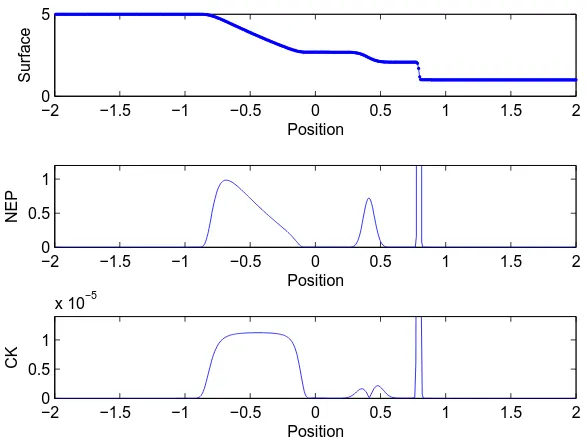
Figure 1. Comparison results using the Rusanov method with 500 cells at time t= 0.2. The first subfigure is the water surface, the second is part of the NEP indicator, and the third is part of the CK weak local residual indicator.
−2 −1.5 −1 −0.5 0 0.5 1 1.5 2
0 5
Surface
Position
−2 −1.5 −1 −0.5 0 0.5 1 1.5 2
0 0.5 1
NEP
Position
−2 −1.5 −1 −0.5 0 0.5 1 1.5 2
0 0.5 1
x 10−5
CK
Position
−2 −1.5 −1 −0.5 0 0.5 1 1.5 2 0
0.5
NEP
Position
−2 −1.5 −1 −0.5 0 0.5 1 1.5 2
0 0.5 1
x 10−6
CK
Position
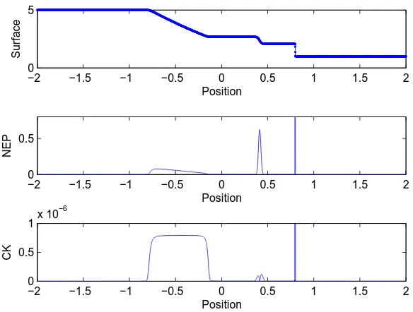
Figure 3. Comparison results using the Rusanov method with 5000 cells at timet= 0.2. The first subfigure is the water surface, the second is part of the NEP indicator, and the third is part of the CK weak local residual indicator.
−2 −1.5 −1 −0.5 0 0.5 1 1.5 2
0 5
Surface
Position
−2 −1.5 −1 −0.5 0 0.5 1 1.5 2
0 0.5
NEP
Position
−2 −1.5 −1 −0.5 0 0.5 1 1.5 2
0 0.5
1x 10 −6
CK
Position
Figure 4. Comparison results using the central-upwind method with 5000 cells at timet= 0.2. The first subfigure is the water surface, the second is part of the NEP indicator, and the third is part of the CK weak local residual indicator.
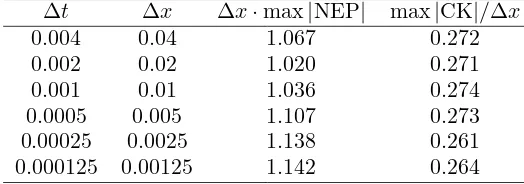
Table 1. The relation between smoothness indicators and the mesh ratio simulated using the Rusanov method at time t= 0.2. Here we take the mesh ratio ∆t/∆x= 0.1.
∆t ∆x ∆x·max|NEP| max|CK|/∆x
0.004 0.04 1.067 0.272
0.002 0.02 1.020 0.271
0.001 0.01 1.036 0.274
0.0005 0.005 1.107 0.273
0.00025 0.0025 1.138 0.261
0.000125 0.00125 1.142 0.264
Table 2. The relation between smoothness indicators and the mesh ratio simulated using the central-upwind method at time t= 0.2. Here we take the mesh ratio ∆t/∆x= 0.1.
∆t ∆x ∆x·max|NEP| max|CK|/∆x
0.004 0.04 1.161 0.280
0.002 0.02 1.125 0.280
0.001 0.01 1.090 0.283
0.0005 0.005 1.084 0.284
0.00025 0.0025 1.157 0.282
0.000125 0.00125 1.093 0.285
We consider the initial condition
q(x, t= 0) =
(5,0,15)t if x <0,
(1,0,5)t if x >0.
(25)
We solve the Ripa model on the domain [−2,2]. The acceleration due to gravity is set to be 1. Uniform space discretisation is used. At time t >0 we obtain three waves, namely the rarefaction, contact, and shock waves.
For the first test we take uniform space grids with 500 cells with the CFL number is 1. We obtain that both NEP and CK indicators detect where rough regions are. However, NEP is better in this case, as CK is oscillatory at around the contact wave. An implementation of CK indicator for this case may give incorrect action when an adaptive method is used to recover the accuracy at around the contact wave. Representative plots of numerical results are given in Figure 1 for the Rusanov method and Figure 2 for the central-upwind method. These Figures 1 and 2 show the water surface and the smoothness indicators at timet= 0.2 simulated using the coarse grids (500 cells), where the smoothness indicators are plotted as their absolute values.
For the second test we take finer uniform space grids with 5000 cells with the CFL number is 1. Again both NEP and CK indicators indicate where rough positions are. However the NEP still performs better in this second case. The CK indicator decays very fast at around the contact wave, whereas the NEP is still able to give a clearer indication where the position of the contact wave is. These results are shown in Figure 3 for the Rusanov method and Figure 4 for the central-upwind method. These Figures 3 and 4 show the water surface and the smoothness indicators at time t = 0.2 simulated using the fine grids (5000 cells), where the smoothness indicators are plotted as their absolute values.
Furthermore we discuss about the performance of the solving methods of the Ripa model. The central-upwind method is less diffusive than the Rusanov method. This is reflected in our simulations. Figure 2 has a sharper shock and a sharper contact wave than those in Figure 1. Furthermore, Figure 4 has a sharper shock and a sharper contact wave than those in Figure 3. In this paper we have considered horizontal topography. Special numerical treatment is needed to deal with non-horizontal topography cases. To compute the NEP for the case of non-horizontal topography, we need to modify the numerical flux formulations, which can be adapted from the work of Mungkasi [9]. To compute the CK indicator for the case of non-horizontal topography, we need to have a well-balanced computation so that the CK indicator behaves correctly, as researched by Mungkasi and Roberts [17].
5. Conclusions
We have proposed the numerical entropy production as a smoothness indicator for numerical solutions to the one-dimensional Ripa model. Numerical results confirm that the performance of the numerical entropy production is better than that of a weak local residual. This suggests that the numerical entropy production is a good candidate for an adaptive indicator to be used in adaptive numerical methods to solve the Ripa model. For future direction, we will implement the numerical entropy production as the refinement indicator in an adaptive mesh finite volume method.
Acknowledgments
The authors thank the two anonymous reviewers for their constructive comments, which helped us to improve the paper.
References
[1] Chertock A, Kurganov A and Liu Y 2014 Central-upwind schemes for the system of shallow water equations with horizontal temperature gradientsNumerische Mathematik127595
[2] Constantin L A and Kurganov A 2006 Adaptive central-upwind schemes for hyperbolic systems of conservation lawsHyperbolic Problems195 (Yokohama: Yokohama Publishers)
[3] Desveaux V, Zenk M, Berthon C and Klingenberg C 2016 Well-balanced scheme to capture non-explicit steady states. Ripa modelMathematics of Computationin press http://dx.doi.org/10.1090/mcom/3069 [4] Ersoy M, Golay F and Yushchenko L 2013 Adaptive multiscale scheme based on numerical density of entropy
production for conservation lawsCentral European Journal of Mathematics111392
[5] Golay F 2009 Numerical entropy production and error indicatorComptes Rendus Mecanique337233 [6] LeVeque R J 1992 Numerical methods for conservation laws (Basel: Birkhauser)
[7] LeVeque R J 2002 Finite-volume methods for hyperbolic problems (Cambridge: Cambridge University Press) [8] Mungkasi S 2013 A study of well-balanced finite volume methods and refinement indicators for the shallow
water equationsBulletin of the Australian Mathematical Society 88351
[9] Mungkasi S 2015 Numerical entropy production of the one-and-a-half-dimensional shallow water equations with topographyJournal of the Indonesian Mathematical Society 2135
[10] Mungkasi S and Roberts S G 2010 A new analytical solution for testing debris avalanche numerical models
ANZIAM Journal52C349-C363
[11] Mungkasi S and Roberts S G 2010 Numerical entropy production for shallow water flowsANZIAM Journal
52C1-C17
[12] Mungkasi S and Roberts S G 2011 A finite volume method for shallow water flows on triangular computational grids Proceedings of The 2011 IEEE International Conference on Advanced Computer Science and
Information System(ICACSIS 2011)79-84
[13] Mungkasi S and Roberts S G 2012 Analytical solutions involving shock waves for testing debris avalanche numerical modelsPure and Applied Geophysics1691847-1858
[14] Mungkasi S and Roberts S G 2012 Approximations of the Carrier-Greenspan periodic solution to the shallow water wave equations for flows on a sloping beachInternational Journal for Numerical Methods in Fluids
69763-780
[15] Mungkasi S and Roberts S G 2012 Behaviour of the numerical entropy production of the one-and-a-half-dimensional shallow water equationsANZIAM Journal 54C18
[16] Mungkasi S and Roberts S G 2013 Validation of ANUGA hydraulic model using exact solutions to shallow water wave problemsJournal of Physics: Conference Series423012029
[17] Mungkasi S and Roberts S G 2014 Well-balanced computations of weak local residuals for the shallow water equationsANZIAM Journal 56C128
[18] Mungkasi S, Li Z and Roberts S G 2014 Weak local residuals as smoothness indicators for the shallow water equationsApplied Mathematics Letters3051
[19] Puppo G 2002 Numerical entropy production on shocks and smooth transitions Journal of Scientific Computing17263
[20] Puppo G 2003 Numerical entropy production for central schemesSIAM Journal on Scientific Computing25
1382
[21] Puppo G and Semplice M 2011 Numerical entropy and adaptivity for finite volume schemesCommunications in Computational Physics101132
[22] Ripa P 1993 Conservation laws for primitive equations models with inhomogeneous layers Geophysical & Astrophysical Fluid Dynamics7085
[23] Ripa P 1995 On improving a one-layer ocean model with thermodynamics Journal of Fluid Mechanics303
169
[24] S´anchez-Linares C, Morales de Luna T and Castro D´ıaz M J 2016 A HLLC scheme for Ripa modelApplied Mathematics and Computation272347