DOI 10.1007/s10640-009-9325-1
A Pollution Offset System for Trading Non-Point Source
Water Pollution Permits
R. A. Ranga Prabodanie ·John F. Raffensperger · Mark W. Milke
Accepted: 23 September 2009 / Published online: 29 October 2009 © Springer Science+Business Media B.V. 2009
Abstract Water pollution from non-point sources is a global environmental concern. Econ-omists propose tradable permit systems as a solution, but they are difficult to implement due to the nature of non-point sources. We present a pollution offset system for trading non-point source water pollution permits. Conventional pollution offset systems suffer from thin mar-kets and transaction costs. In this paper, we show how to overcome these problems with a centrally managed common-pool market. We define permits as allowable nitrate loading to a groundwater aquifer. This trading system utilizes estimates of potential nitrate leaching from land uses, a set of transport coefficients generated from a simulation of nitrate transport in groundwater, an online trading system, and a linear program to clear the market. We illustrate the concept using a hypothetical case study.
Keywords Nitrate·Non-point sources·Linear program·Trading· Water pollution permits
1 Introduction
A hundred years ago, the main sources of water pollution were untreated human wastes and industrial discharges. Industrialized nations now control these point sources through treat-ment and disposal technologies, and pollution laws (Revenga and Mock 2000). Nevertheless, even the developed world suffers from non-point (diffuse source) pollution caused mainly by intensive agriculture.
R. A. R. Prabodanie (
B
)·J. F. RaffenspergerDepartment of Management, University of Canterbury, Private Bag 4800, Christchurch 8140, New Zealand
e-mail: [email protected] M. W. Milke
Nitrate is a major agricultural non-point source pollutant. Synthetic fertilizer, manure, and livestock effluents contain nitrogen in different forms as nitrate, ammonia, ammonium, urea, amines, or proteins. Once applied on soil, nitrogen may be taken up by plants, carried away by surface runoff, or transformed into nitrate and leach into groundwater. Nitrogen loading into water bodies usually occurs as nitrate leaching into the groundwater system rather than as surface runoff. Excess nitrates in water can cause severe threats to human health and aquatic ecosystems.
National and international environmental authorities have set water quality standards (or maximum acceptable levels of pollution) to meet human and ecosystem health needs. New Zealand’s national drinking water guideline for nitrate is 50 mg/l. In New Zealand’s Waikato region, groundwater nitrate levels commonly exceed this level due to intensive mar-ket gardening and livestock farming (Environment Waikato 2008). In the United States, most shallow groundwater aquifers in agricultural areas have high nitrate concentrations (U.S. Geological Survey 1999).
Tradable permit systems have been proposed as a means of controlling water pollution from commercial sources such as dairies and crop farms. The main benefits of trading sys-tems are the ability to reveal the economic values of the discharge rights and to shift them from low value uses to high value uses. For commercial land users, tradable pollution permit systems provide additional flexibility in land use decisions.
However, defining, pricing and trading of non-point source water pollution permits require measurement of pollutant leaching and runoff losses from the soil and tracing of fate of pol-lutants in groundwater. The pollutant flow paths, attenuation during the flow, and time lags between the discharge and appearance at a water body depend on catchment hydrogeology and climate. Different sources affect a given receptor (a water body or a point on a water body where water quality is monitored) with different intensities and timings, so one-to-one bilateral trade can worsen water quality at some receptors. The key requirement to facilitate trade in non-point source water pollution permits is the ability to relate the source loading to the time varying impacts on water quality of hydro-geologically connected water bodies at different receptors (Morgan et al. 2000;O’Shea 2002). Hence, a non-point source water pol-lution trading system needs hydrological modelling and a central authority to facilitate and oversee trading. The central authority also needs a well-defined methodology to determine the equilibrium prices and allocations.
This paper is specifically about nitrate leaching into groundwater. The term “nitrate per-mit” will refer to a water pollution permit, which allows a specified amount of nitrate leaching (loading) into a groundwater aquifer. We use hydrological simulations to obtain a set of coef-ficients which describe the relationships between the source loading and quality deterioration at receptors.
2 Pollution Permit Trading: Theory and Application to Water Pollution
Coase(1960) was the first to propose a market mechanism as a means of dealing with eco-nomic externalities.Dales(1968) demonstrated the applicability of trading solutions to the specific problem of water pollution.Montgomery(1972) provided the theoretical foundation for trading pollution permits, introducing “diffusion coefficients” to relate source emissions to receptor pollutant concentrations. Montgomery discussed an “ambient” permit system in which an authority issues permits for each receptor separately. Sources must maintain a port-folio of permits to match impacts on each receptor. Montgomery’s system suffered from high transaction costs, soKrupnick et al.(1983) proposed a pollution offset system. A pollution offset system needs an environmental quality model to simulate the impact of each proposed transaction and ensure that it does not cause quality standards to be violated at any receptor. McGartlend and Oates(1985) presented a modified offset system by introducing redefined quality standards to the original offset system.McGartland(1988) argued that the ambient permit and pollution offset systems are equivalent under perfect competition, and a competi-tive equilibrium exists, but there are obstacles in reaching this equilibrium. He suggested that brokers could help overcome these obstacles. Brokering was further developed byErmoliev et al.(2000), who identified the need for multilateral trade in pollution permits. They sug-gested that an environmental agency, acting as a Walrasian auctioneer, could coordinate the trade among decentralized agents submitting bids and offers online.
Though much of the economic theory appears to be established, actual water pollution permit trading is mostly limited to a few point source trades (King and Kuch 2003). The lit-erature is dominated by point source emission or ambient permit trading systems (Neil et al. 1983;Eheart et al. 1987;Leston 1992;Weber 2001;Hung and Shaw 2005). We discuss three types of non-point source discharge permits trading system proposed to date: an ambient permit system, a trading ratio system and a zonal permit system.
Morgan et al.(2000) seem to be the first to present a method for trading non-point source permits. They propose an ambient permit system for trading nitrate discharge permits. It consists of three parts: (1) a production model that estimates the profits from different pro-duction practices (crop rotation and fertilizer application rate), (2) a soil model that estimates the water and nitrogen leaching from each practice, and (3) a groundwater model that sim-ulates the nitrate movement in groundwater. An auctioneer finds a price for each receptor which satisfies the water quality standards and balances demand and supply. This system is best suited when there is only one receptor, as a separate auction is needed for each receptor. Even for one receptor, a large number of auction rounds may be needed to clear the market. Horan et al.(2002) designed a system for trading nitrogen permits, including point and non-point sources. A trade between two source categories is based on a trading ratio, deter-mined so that pollution does not increase because of trade. The model does not include explicit water quality standards, but rather an economic cost of pollution. Thus, their system requires knowledge of the cost of pollution to the rest of society, and has no constraints associated with the sustainability of the environment.
for each type of permit. This zonal permit system is applicable only when there is a single receptor point.
Ambient permit systems suffer from high transaction costs due to maintaining a portfolio of permits and having several markets (Ermoliev et al. 2000). They usually work well with one or few receptors. Even with a single receptor, non-point sources usually have impacts over different time scales. Consequently, different types of permits must be defined in terms of the time of impact. These temporal impacts again create many markets. If the impacts last for more than one time step, a source may need a portfolio of permits to cover operation in a single year. Hence, there are significant difficulties in starting and operating ambient permit systems for non-point source pollution, and simplifications can lead to undesirable impacts on water quality.
The outcomes of trading ratio systems depend on how the administrator selects the trad-ing ratios, and no proven method exists to find the right tradtrad-ing ratios for non-point source trading systems. On the other hand, zonal permit systems are hard to apply to catchments with many receptors. When zones are defined in terms of only one parameter, for example lag time, other factors such as spatial variation in attenuation may not allow the trading system to achieve all potential benefits of trade.
As our literature survey reveals, none of the prior work has attempted a pollution offset system for trading non-point source water pollution permits, possibly due to the need for environmental simulations and the understandable fear of thin trading from high transac-tion costs. We propose a pollutransac-tion offset system, supported by hydrological, economic and optimisation models, with the potential to overcome those issues.
3 Methodologies: Designing a Pollution Offset System
The proposed nitrate permit trading system is a type of pollution offset system, applicable at the catchment scale. It consists of four components. First, a leaching loss model estimates nitrate leaching to the aquifer from potential land uses and thus the size of the permit required for each land use option. Based on permit requirements and profitability of land use options, land users choose their individual demand and supply relative to an initial allocation of per-mits. Second, a contaminant transport model provides a matrix of transport coefficients which quantify the relationship between source loading and pollution effect at the receptors. Third, a centrally controlled electronic market facilitates trade by accepting bids and offers from land users. Fourth, a linear program determines the optimal trades based on the source-receptor relationships and land user demand and supply. Below, we provide a detailed description of each component and its contribution.
3.1 Leaching Loss Model
A regional environmental authority acts as a facilitator of trade. We assume that the author-ity can identify the potential land use options, and can estimate nitrate leaching from each option. In New Zealand, most environmental authorities have tools (e.g., Overseer, FarmSIM, and NPLAS) to estimate leaching. If those tools were available to the users, they could esti-mate the leaching from intended operations themselves. In any case, a single official estiesti-mate is needed for the market.
Nitrate leaching, and therefore the nitrate permits, can be specified in two equivalent ways.
1. Mass nitrate leaching to the aquifer below the land area, as mass leaching per land area per period, kg/ha/year.
2. Nitrate concentration of the water leaching to the aquifer (recharge) from the land area, mg/l.
In this paper, we use the first method and specify the permits in kg/ha/year, but the difference is only a change of units.
3.2 Nitrate Transport Model
In the second component, we establish the numerical relationship between source loading and level of water pollution at each receptor, represented by a matrix of transport coefficients. The transport coefficients are synonymous with the diffusion coefficients discussed in the prior work on both air and water quality trading systems, with one key difference: coefficients used previously had only two indices, source and receptor, but the transport coefficients used here have a third dimension of time. The transport coefficients may be defined in several equivalent ways.
1. The concentration at a receptor, at a given time, from one unit of leaching at a pollution source during a certain time period (measured in concentration units, e.g., mg/l, and used with receptors such as groundwater wells).
2. The mass pollutant flux at a receptor, at a given time, from one unit leaching at a pollution source during a certain time period (measured in flux units, e.g., kg/day, and used with receptors such as streams).
3. The mass pollutant input to a receptor during a given time period, from one unit leaching at a pollution source during a certain time period (measured in mass units, e.g., kg, and used with receptors such as lakes).
To estimate the transport coefficients, we simulate the contaminant transport based on the hydro-geological properties of the catchment, using commonly available computer codes. Some software tools used to simulate groundwater flow and contaminant mobility in ground-water are MODFLOW (Harbaugh et al. 2000), MT3D (Zheng 1990) and MODFLOW GWT (U.S. Geological Survey 2006).
The simulations treat leaching as contaminated recharge, and quantify source load-ing as the pollutant leachload-ing into the model cells (zone) which represent the aquifer be-low the source (e.g., farm). We can therefore simulate unit leaching from each sourcei
to obtain its impact on the concentration, flux or mass at each receptor j, at each time stept of interest. Each of these values fills an entry [i,j,t] of the transport coefficient matrix.
trading, so we have to estimate their contribution at each receptor. We can simulate the non-tradable sources using the same contaminant transport model and obtain the concentration, flux or mass that occurs at each receptor, at each time step of interest. These non-tradable source contributions and the water quality standards together determine the availability of nitrate permits to be distributed via trading.
3.3 The Online Trading System
The third component to our system is a centrally controlled online trading system which brings buyers and sellers together and facilitates multilateral trade. Initial permits are allo-cated to land users, who are then allowed to trade through a web interface. Traders do not trade with each other pair-wise, but rather buy from and sell to the centrally-controlled mar-ket. We suggest that a regional environmental authority is the best candidate to oversee the trading system. We call the person or the institution who oversees the market as the “market manager.”
Each user calculates their demand or supply at each possible permit price, based on the potential profit from each land use option and the cost or revenue from buying or selling the nitrate permits required for each land use option. Then users submit bids and offers to the online trading system as a series of price and quantity (buy or sell) pairs. These bids and offers define every user’s demand function for nitrate permits.
Clearing the market is complicated by many factors. First, users are bidding for permits that have different impacts on the water quality constraints concerned. Therefore, the bids are not comparable between traders. Second, the usual criteria of accepting the highest bids and lowest offers is not applicable in this case because the acceptance of the highest bid may violate the water quality standards. Instead, to clear the market, the market manager must find a (potentially different) price for every source, so that demand matches hydrology-adjusted supply, quality meets requirements at all receptors at all times, and social benefit achieves the maximum. As a means of dealing with the complexity, we use a linear program to clear the market. Linear programs have been successfully used for this purpose in complicated multilateral trading situations such as electricity markets (Hogan et al. 1996). We give the linear program below in Sect.3.4.
The market manager runs the linear program and displays the calculated allocations and prices on the trading system web. A few tentative rounds of market clearance may be helpful for the participants to generate expectations about the results and finalise the bids. Once the market is officially cleared (final clearance), the market manager collects money from sellers, pays the buyers, and clears the market. Buyers pay and sellers receive a specific price assigned to each. There is no matching of buyers and sellers, as everyone trade through a common pool. The prices need not match, and total purchases need not to equal total sales, as the permits are not directly comparable.
3.4 Linear Program
The final component in our trading system is the linear program, which will determine the prices and allocations that maximise total consumer and producer surplus, subject to water quality standards and initial permit allocations.
Consumer and producer surplus, or more exactly buyer and seller surplus in this case (since no-one “consumes” pollution), measure the benefit that buyers and sellers derive from participating in a market. Maximum social benefit is achieved when the sum of buyer and seller surplus is maximised, assuming that participants have submitted truthful bids. We calculate the buyer and seller surplus from the bids and offers submitted by the traders.
We assume that permits are short term property leases rather than long term property own-ership rights. Though a permit is valid for a short period, the effects exist for longer periods. Trades are feasible if water quality standards are expected to be met while the permits are valid and in the future following expiration. Hence, the planning horizon should be long enough to capture the impacts of all sources on all receptors. We divide the planning horizon into steps and impose water quality standards at every step. The length of each time step should be short enough to guarantee that the quality standards are met continuously and long enough to avoid a large number of redundant water quality constraints in the linear program. To convert the water quality requirements into mathematical constraints, we assume a linear relationship between leaching and the quality deterioration at each receptor at every time step. By assuming linearity, we can calculate the nitrate concentration, flux or mass at any receptor as the sum of contributions from all sources. This is a commonly applied assumption in solving groundwater management problems (Morgan and Everett 2005).
Indices
i=1, . . .,Ntraders.
j=1, . . .,Mreceptors.
t=1, . . .,T time periods.t =1 indicates the current period. The planning horizon isT
periods, meaning water quality constraints apply fort =1, . . .,Tperiods. The permits are valid only fort=1, . . .,t′periods(t′<T).
k=1, . . .,K bids or offer steps. Each trader can submit up toK bid or offer steps.
Parameters
Ai = initial allocation to traderi.
Hi j t = the concentration, flux or mass that occurs at receptor j, at timet, from one
unit leaching at pollution sourcei,duringt =1, . . .,t′(nitrate permits are valid during
t=1, . . .,t′<T).
Cj t = the total concentration, flux or mass at receptorj, at timet, from all non-tradable
sources.
Sj t = the maximum acceptable concentration, flux or mass at receptor jat timet.
Ui k = upper bound onkth bid step placed by traderi(positive for buy steps and negative
for sell steps).
Pi k = price ofkth step placed by traderi.
Decision variables
bi k = purchases/sales by traderifromkth bid/offer.
qi = maximum leaching allowed for traderiduringt =1, . . .,t′. This is the size of the
permit held by traderiafter market clearing.
Objective function
MaximiseikPi kbi k, subject to
Upper bounds on bids and offers
IfUi k≥0,0≤bi k ≤Ui k,elseUi k≤bi k≤0 for alli=1, . . .,N and
k=1, . . .,K(1)θi k
Compliance constraints
qi−
k
bi k= Ai for alli=1, . . .,N (2)µi
Water quality constraints
i
Hi j tqi ≤Sj t−Cj t for all j =1, . . .,Mandt=1, . . .,T (3)λj t
Other constraints
qi ≥0 for alli=1, . . .,N (4)βi
The right-hand side of each water quality constraint,Sj t−Cj tindicates the net amount of
pollution capacity at receptor jin periodt, available for allocation through trading. We can estimate expected values forCj tusing the same transport simulation model discussed above.
However, determiningSj tshould be done carefully. Water quality standards usually specify
the maximum acceptable mass pollutant discharge into a water body during a period or the maximum acceptable concentration at a time. If we setSj tequal to those standards, and some
constraint for yeart0becomes binding in the solution, we may not be able to allocate any
permit that affects periodt0in the future. We are currently studying the optimal method to
determineSj t which is a problem of resource allocation over time. In this work, we assume
thatSj t−Cj tis given by the catchment authority, as the total amount of resource available
for allocation via trading.
The variables listed in the right hand side of the constraints,θi k, µi, λj t, andβi are the
shadow prices associated with the constraints. The shadow price of each trader’s compliance constraint,µiindicates the cost to society if the trader were given an additional 1 kg/ha/year
permit. We suggest that this price is correct, following theory of marginal cost pricing. From the dual formulation of the above linear program, we can show that the individual participant price,µi = j
tHi j tλj t, whereλj t is the market value of a unit increase
in nitrate concentration, flux or mass at receptor j in time periodt. The above relationship indicates that the price of sourceiis determined by its impacts on all the receptors over the planning horizon. From the dual formulation, we may also prove that the participant price,
µi is at least the offer/reservation price or a better price if the bid/offer is selected.
4 Illustration
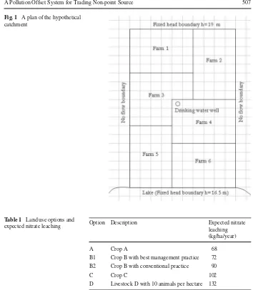
Fig. 1 A plan of the hypothetical catchment
Table 1 Land use options and
expected nitrate leaching Option Description Expected nitrateleaching (kg/ha/year)
A Crop A 68
B1 Crop B with best management practice 72 B2 Crop B with conventional practice 90
C Crop C 102
D Livestock D with 10 animals per hectare 132
1. The mass nitrate input to the lake in every year is below the predetermined standard, 4 tonnes per year. Nitrate, once in the lake, does not reside there for more than a year. 2. The nitrate concentration of the drinking water well does not exceed 50 mg/l at any time.
The catchment has two receptors, the lake (j=1) and the well (j=2). Taking into account the two water quality standards and expected non-tradable source contributions including the nitrates already in the aquifer, the regional environmental authority has informed the market manager that in the current instance of trading, he should allocate only 1/8th of the environmental standards. Hence,S1t−C1t =5000 kg andS2t −C2t =6.25 mg/l for allt,
for this problem.
4.1 A Trading System to Allocate Nitrate Permits
catchment is approximately 40–50 years and we consider a 40 year planning horizon. During this planning horizon, trading would occur and the market will be cleared eight times. We will discuss the results of the first instance of trading.
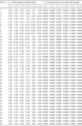
We simulated groundwater flow with MODFLOW and nitrate transport using MT3D. Some hydro-geological data used in the models are given in the appendix. Using the nitrate transport model, we simulated 1 kg/ha/year nitrate leaching from each farm and obtained the transport coefficientsHi j tshown in Table2.
We assume that all non-point sources get the same initial allocation as a rate of loading in kg/ha/year. We calculated the maximum feasible initial allocation from a simple linear pro-gram, which maximised initial allocation subject to water quality standards. The calculated initial allocation was 77.447 kg/ha/year for every farm (Ai =77.447 for alli). The binding
water quality constraint which determined this initial allocation was the well concentration constraint for year 5: 0.0236q1+0q2+0.0398q3+0.0173q4+0q5+0q6 ≤ 6.25. An initial allocation which binds a single constraint implies that only one constraint is fully allocated initially. We discuss the consequences of such initial allocation in the next section on outcomes of trade.
With this free initial allocation of permits, farms can adopt only options A or B1. If trade is allowed, farms can adopt other options. If a farm selects option A for the next 5 years, it can sell up to 9.447 kg/ha/year of the permit. Similarly, if a farm selects option B1, it can sell up to 5.447 kg/ha/year. If a farm wishes to adopt land use option B2, it has to buy at least 12.553 kg/ha/year. Similarly, if any farm needs to adopt land use option C or D, it has to buy at least 24.553 kg/ha/year or 54.553 kg/ha/year respectively. Based on the initial allo-cation, the permit requirements, and profitability of land use options, the farms choose bids and offers which maximise their profits, each assuming that they cannot influence market price.
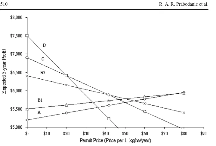
Our market design does not need to address the user’s optimization problem. This trad-ing system is not a decision support system for individual farmers, as farmers make their own production decisions given permit prices. However, to understand how the farmers will arrive at the bids/offers, assume that a farmer’s potential five year profit from crop A, crop B, crop C, and livestock D are $5200, $6400, $6900, and $7500 respectively. Assume the best management practice for crop B costs $900.
The graphs in Fig.2show how this farmer’s 5-year profit from each farming option would vary with the permit price. If the price is $20 or less, option D is most profitable. This farmer would buy 54.553 kg/ha/year at $20/kg/ha/year or at a lesser price. If the price is greater than $20 but less than $41.67, option C is most profitable, and the farmer would buy 24.553 kg/ha/year. If the price is above $41.67 but below $50, option B2 is most profitable and the farmer would buy 12.553 kg/ha/year. If the price is over $50 but below $75, B1 is the most profitable option and the farmer would sell 5.447 kg/ha/year. If the price is over $75, option A is most profitable and the farmer would sell 9.447 kg/ha/year.
Table 2 Mass nitrate input to the lake (kg) and concentration in the well (mg/l) that occurs due to 1 kg/ha/year leaching from each farm during the first 5 years (Transport Coefficients,Hi j tforj=1 andj=2) Year (t) j=1 (nitrate input to the lake in kg) j=2 (concentration occurs in the well in mg/l)
i=1 i=2 i=3 i=4 i=5 i=6 i=1 i=2 i=3 i=4 i=5 i=6
Fig. 2 Profitability of land use options vs. permit price
Table 3 Submitted bids and offers
Permit price Most profitable option Extra permit required (+) or available (−) (kg/ha/year)
Bid/Offer
Price Quantity (kg/ha/year)
Below $20.00 D 54.553 $20.00 30.000
$20.00–$41.66 C 24.553 $41.00 12.000
$41.67–$49.99 B2 12.553 $49.00 12.553
$50.00–$74.99 B1 −5.447 $50.00 −5.447
Above $75.00 A −9.447 $75.00 −4.000
Table 4 Permit allocations and prices determined by the linear program Source,i Buy/sell,bi
(kg/ha/year)
Final qty,qi
(kg/ha/year)
Price, µi
Payments/ receipts
End land use
Farm 1 17.516 94.963 $41.00 $718.16 Crop B
Farm 2 54.553 132.000 $2.27 $123.83 Livestock D
Farm 3 −9.447 68.000 $76.01 −$718.08 Crop A
Farm 4 −2.160 75.287 $50.00 −$107.98 Crop B with BMP
Farm 5 24.553 102.000 $31.36 $769.96 Crop C
Farm 6 12.871 90.318 $41.00 $527.71 Crop B
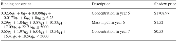
Table 5 Binding constraints in the linear programming solution
Binding constraint Description Shadow price
0.0236q1+0q2+0.0398q3+
0.0173q4+0q5+0q6≤6.25
Concentration in year 5 $1708.97 0.29q1+1.04q2+3.87q3+10.33q4+
17.09q5+22.71q6≤5000
Mass input in year 6 $1.52 0.65q1+1.97q2+6.04q3+13.54q4+
15.41q5+18.56q6≤5000
Concentration in year 7 $0.53
4.2 Outcomes of Trade
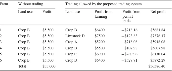
The results indicate that every farm is better off after trade. If trade is not allowed, all farms can grow only crop A or crop B which are least profitable. As a result of trading, farms 2 and 5 can farm livestock D and crop C which are most profitable. Farms 1 and 6 can save a large portion of the cost of best management practice by buying more permits. Farms 3 and 4 can make additional profit by farming crop A and crop B and selling the extra permits.
According to the results of trading listed in Table4, buyers and sellers get at least their reservation price or better. Even though bids are identical, prices vary by location. The reason is that leaching at some locations has a greater impact on the binding constraints than leaching at other locations. The binding constraints were the well concentration constraint in year 5, mass nitrate input constraint in year 6, and mass nitrate input constraint in year 7, as listed in Table5. Farm 3 has the highest price because it has the greatest impact on the well con-centration in year 5 (0.0398 mg/l) which has the highest shadow price. Farm 2 has the lowest price because it has zero impact on the binding constraint with the highest shadow price and relatively small impacts on the others (1.04 and 1.97 kg).
As the permits are defined on a per hectare basis, the prices depend on the farm size as well. Therefore, prices may not be comparable among the farms if the farm sizes (areas) vary significantly, which is not the case in this example (as shown in Fig.1, the areas of farms 1, 3, 4, and 6 are equal to 30 ha while farms 2 and 6 are 32 and 28 ha respectively). In any case, comparable farm prices could be obtained by dividing the individual farm price by the area. The total payment due to sellers is less than the total paid by buyers. As a result, the market manager gets a surplus of $1313.60. This surplus is explained by the binding water quality constraints. The constraints for mass nitrate inputs in years 6 and 7 were not binding in the initial allocation (were not fully allocated initially), but becomes binding after trade (fully allocated after trade). These two constraints can be viewed as initially under-allocated resources where the market manger has kept aside 5000−(0.29×77.447+1.04×77.447+ 3.87×77.447+10.33×77.447+17.09×77.447+22.71×77.447)=714.56 kg of one resource and 5000−(0.65×77.447+1.97×77.447+6.04×77.447+13.54×77.447+15.41× 77.447+18.56×77.447)=649.42 kg of the other. The buyers first buy from the market man-ger who sells his 714.56 kg of the first resource at the shadow price of the constraint, $1.52 and his 649.42 kg of the other resource at the shadow price of the constraint, $0.35. The surplus money left after clearing the market is the buyer’s payment for the resources they bought from the market manager, 714.56×$1.52+649.42×$0.35=$1313.00=surplus money left.
Table 6 Potential gains from trade
Farm Without trading Trading allowed by the proposed trading system Land use Profit Land use Profit from
farming
Profit from permit trade
Net profit
1 Crop B $5,500 Crop B $6400 −$718.16 $5681.84
2 Crop B $5,500 Livestock D $7500 −$123.83 $7376.17
3 Crop B $5,500 Crop A $5200 $718.08 $5918.08
4 Crop B $5,500 Crop B $5500 $107.98 $5607.98
5 Crop B $5,500 Crop C $6900 −$769.96 $6130.04
6 Crop B $5,500 Crop B $6400 −$527.71 $5872.29
Total $33,000 $36586.40
Non-point source water pollution permits may be considered as a bundle of constraint rights where a constraint right is a right to increase the pollutant concentration, flux, or mass at a certain receptor in a certain time period (similar to ambient permits). Therefore, the permits may be broken up into constraint rights and each constraint may be fully allo-cated (independently without looking at other constraints) among the sources as an initial allocation (McGartlend and Oates 1985). Then after the market is cleared, the individual payments/receipts should be calculated from the shadow prices of the constraints and the amounts of constraint rights purchased and sold.
The total bought, 109.493 kg/ha/year, does not match the total sold, 11.606 kg/ha/year, because the transport coefficients are different, and the permits are not comparable among farms. The quantities sold by farm 3 and farm 4 are 9.447 and 2.160 kg/ha/year. These permits, if not sold, contribute to the well concentration in year 5 by 0.0398×9.447+0.0173×2.160= 0.413 mg/l. This equals the contribution of the 109.493 permits bought by farms 1, 2, 5 and 6 (0.0236×17.515+0×54.553+0×24.553+0×12.871= 0.413 mg/l). The linear program rescales quantities so that the effects at the receptors remain feasible.
If farm 1 raised the price of his last three bids from $20, $41, and $49 to $50 each in order to buy more, then the result will be buying 19.926 kg/ha/year, at $50 each. The farmer will be penalized by a higher price. Even though farm 1 is prepared to pay more, it cannot buy more because it has a significant impact on the water quality constraints.
Potential profits with and without trade are calculated in Table6. Every farm can make more profit if trade is allowed. Without trade, the potential profit for farmers is $33,000. If trade is allowed, they can make a higher profit of $36,586.
We simulated the nitrate loadings from the optimal permit allocation to verify that water quality standards were met in all periods. This verifying simulation may fail if the assumption of linearity were not true.
5 Discussion and Conclusions
The major criticism of pollution offset systems is that they have thin trading. A proposed pair-wise transaction may be infeasible because it violates quality standards. Even if simu-lation results allow a transaction, with one or two user-quantity changes at a time, the cost of the simulation itself raises the overall transaction cost considerably. By contrast, the pro-posed system facilitates multilateral trade. It provides higher potential for offsetting impacts from one user by adjusting quantities of multiple sellers simultaneously, and also avoids the need to simulate every user’s transaction. The physical leaching and contaminant transport models determine coefficients for the linear program, which then chooses the optimal trades. Therefore, the use of physical models is one-off rather than for every transaction.
Because prices and allocations depend on the bids/offers and water quality constraints, this trading system should result in an economically optimal and environmentally feasible distribution of nitrate permits. Participants do not need to find trading partners because they buy from and sell to a common pool. They do not have to negotiate with affected parties, as the model manages impacts on all third parties and the environment. Information such as price history can be displayed freely on the trading system web. Therefore, the proposed trading system incurs almost no transaction costs. While we have demonstrated the system for nitrate, it is applicable for trading water pollution permits defined for any hydrological pollutant.
The outcomes of the proposed trading system depend on the accuracy of the transport coefficients. Market implementers should use well-calibrated hydrological models to deter-mine these coefficients but, even if calibration is poor, our system would use existing data better than any other existing allocation system. The outcomes also rely on compliance to the land use practices allowed by the permits. Enforcement issues are beyond the scope of this paper.
Strategic behaviour may be possible and remains to be studied. In any case, whatever the offer price, whether users collude or attempt to game the system, water quality constraints still restrict the quantity bought (unless users break market rules outright). Therefore, strate-gic behaviour at worst would result in inefficient transfers between users. A user who wished to game the system (say, by buying all rights in the catchment in order to create a monopoly) would be heavily burdened by the local nature of the impacts, as determined by the transport coefficients.
The proposed trading system can attain efficient allocation of permits if the participants bid truthfully and do not behave strategically.Montero(2008) has presented an interesting work on mitigating strategic behaviours. He presented a modified sealed-bid auction for an endogenous number of permits including a system of paybacks or rebates to encourage the participants to bid truthfully. Montero’s auction results in an efficient allocation of permits even if the participants collude and the total number of permits is fixed as in the case of water pollution permits. He has applied the auction to a water pollution problem in a river with five point sources, for a single period and single receptor. However, non-point sources have effects many periods into the future, and catchment managers may wish to consider multiple recep-tors. Therefore, Montero’s system would need extensions to apply to the general non-point source water pollution problem.
pollutants in groundwater last longer than atmospheric pollution, so our system requires a much longer planning horizon.
We are extending this trading system to include both point and non-point sources. Other future work includes considering overland runoff, uncertainty aspects of the non-tradable source contributions, nutrient reducting land uses such as wetlands, and better methods of resource allocation over a very long planning horizon. Application of this trading system to a real agricultural catchment will help further evaluation of the system.
Appendix: Model Parameters Used with MODFLOW and MT3D Simulations
Horizontal hydraulic conductivity: 0.0006 m/s Vertical hydraulic conductivity: 0.0003 m/s Storage coefficient: 0.0001 1/m
Porosity: 0.15
Recharge: 100 mm/year Longitudinal dispersivity: 10 m
Ratio, horizontal to longitudinal dispersivity: 0.1 Ratio, vertical to longitudinal dispersivity: 0.01 Distribution coefficient: 1×10−71/(mg/l)
Aquifer thickness: 20 m
Model cell size: 100m×100m×20m
References
Coase RH (1960) The problem of social cost. J Law Econ 3(1):1–44 Dales JH (1968) Land, water and ownership. Can J Econ 1(4):791–804
Eheart JW, Brill ED, Lence BJ, Kilgore JD, Uber JG (1987) Cost efficiency of time-varying discharge permit programs for water quality management. Water Resour Res 23(2):245–251
Environment Waikato (2008) Nitrate contamination of groundwater. Retrieved 26 December 2008, fromhttp://www.ew.govt.nz/Environmental-information/groundwater/Monitoring-groundwater-quality/ Nitrate-contamination-of-groundwater/
Ermoliev Y, Michalevich M, Nentjes A (2000) Markets for tradable emission and ambient permits: a dynamic approach. Environ Resour Econ 15(1):39–56
Harbaugh BAW, Banta ER, Hill MC, McDonald MG (2000) MODFLOW-2000: The U.S. Geological Survey Modular Groundwater Model. U.S. Geological Survey
Hogan WW, Read EG, Ring BJ (1996) Using mathematical programming for electricity spot pricing. Int Trans Oper Res 3:243–253
Horan RD, Shortle JS, Abler DG (2002) Point-nonpoint nutrient trading in the susquehanna river Basin. Water Resour Res 38(5):8:1–8:12
Hung MF, Shaw D (2005) A trading-ratio system for trading water pollution discharge permits. J Environ Econ Manage 49(1):83–102
Kerr S, Rutherford K, Lock K (2007) Nutrient trading in Lake Rotorua: goals and trading caps. Motu Economic and Public Policy Research
King DM, Kuch PJ (2003) Will Nutrient Credit Trading Ever Work? An assessment of supply and demand problems and institutional obstacles. Environmental Law Reporter. News and Analysis, 5-2003 Krupnick A, Oates W, Verg EVD (1983) On marketable air pollution permits: the case for a system of pollution
offset. J Environ Econ Manage 10:233–247
Leston D (1992) Simulation of a two-pollutant, two-season pollution offset system for the Colorado river of Texas below Austin. Water Resour Res 28(5):1311–1318
Martin KC, Joskow PL, Ellerman AD (2007) Time and location differentiated NOx control in competitive elec-tricity markets using cap-and-trade mechanisms. Center for Energy and Environmental Policy Research McGartland A (1988) A comparison of two marketable discharge permit systems. J Environ Econ Manage
15:35–44
McGartlend AM, Oates WE (1985) Marketable permits for prevention of environmental deterioration. J Envi-ron Econ Manage 12:207–228
Montero JP (2008) A simple auction mechanism for the optimal allocation of the commons. Am Econ Rev 98(1):496–518
Montgomery WD (1972) Markets in licenses and efficient pollution control programs. J Econ Theory 5(3):395–418
Morgan DS, Everett R (2005) Application of simulation-optimization methods for management of nitrate loading to groundwater from decentralized wastewater treatment systems near La Pine, Oregon. US Geological Survey Oregon Water Science Centre
Morgan CL, Coggins JS, Eidman VR (2000) Tradable permits for controlling nitrates in groundwater at the farm level: a conceptual model. J Agric Appl Econ 32(2):249–258
Neil WO, David M, Moore C, Joeres E (1983) Transferable discharge permits and economic efficiency: the Fox River. J Environ Econ Manage 10(4):346–355
O’Shea L (2002) An economic approach to reducing water pollution: point and diffuse sources. Sci Total Environ 282(283):49–63
Revenga C, Mock G (2000) Dirty water: pollution problems persist. World Resources Institute
U.S. Geological Survey (1999) The quality of our nation’s waters: nutrients and pesticides. U.S. Geological Survey
U.S. Geological Survey (2006) Data input instructions for groundwater transport process (GWT). Reston, Virginia