Aquatic Geochemistry 9: 1–17, 2003.
© 2003Kluwer Academic Publishers. Printed in the Netherlands. 1
Analysis of the Major Fe Bearing Mineral Phases in
Recent Lake Sediments by EXAFS Spectroscopy
LORENZO SPADINI1, MARKUS BOTT2, BERNHARD WEHRLI2,⋆ and
ALAIN MANCEAU1,3
1Environmental Geochemistry Group, LGIT-IRIGM, University of Grenoble and CNRS, BP 53, 38041 Grenoble France Cedex 9;2Swiss Federal Institute for Environmental Science and Technology (EAWAG) and Swiss Federal Institute of Technology (ETH), Limnological Research Center CH-6047 Kastanienbaum, Switzerland;3Present address: Hilgard Hall #3110, University of California, Berkeley, CA 94720-3110 USA
(Received: 26 August 2002; accepted: 1 August 2003)
Abstract. Extended X-ray absorption fine structure (EXAFS) spectroscopy and chemical analyses were combined to determine the Fe bearing minerals in recent lake sediments from Baldeggersee (Switzerland). The upper section of a laminated sediment core, deposited under eutrophic conditions, was compared to the lower part from an oligotrophic period. Qualitative analysis of FeK EXAFS agreed well with chemical data: In the oligotrophic section Fe(II)–O and Fe(III)–O species were present, whereas a significant fraction of Fe(II)–S sulfides was strongly indicated in the eutrophic part. A statistical analysis was performed by least square fitting of normalized reference spectra. The set of reference minerals included Fe(III) oxides and Fe(II) sulfides, carbonates and phosphates. In the oligotrophic regime no satisfying fit was obtained using the set of reference spectra, indicating that siderite (FeCO3) was not present in a significant amount in these carbonate-rich sediments. Simulated EXAFS spectra for a (Cax, Fe1−x)CO3solid solution allowed reconstructing the specific
features of the experimental spectra, suggesting that this phase was the dominant Fe carrier in the oligotrophic section of the core. In the eutrophic part, mackinawite was positively identified and represented the dominant Fe(II) sulfide phase. This finding agreed with chemical extraction, which indicated that 18–40 mol% of Fe was contained in the acid volatile iron sulfide fraction. EXAFS spectra of the eutrophic section were best fitted by considering the admixture of mackinawite and the Fe–Ca carbonate phase inferred to be predominant in the oligotrophic regime.
Key words:acid volatile sulfides, EXAFS, iron carbonates, iron sulfides, lake sediments, mackinaw-ite, selective extraction, solid solution, speciation
1. Introduction
In complex environmental systems like soils, aquifer material and sediments iron is typically present as a mixture of different mineral phases. Dissolution and precip-itation of iron minerals are controlled by redox conditions and different microbial and geochemical processes (Davison, 1993; Burdridge, 1993; Cornell and Schwert-mann, 1996; Hansel et al., 2001; Mettler et al., 2001). There is a considerable
interest to analyze the dominant mineral form of iron present in these environ-ments. Important parameters such as the adsorption capacity or the bioavailability for iron reducing organisms depend on the mineral phase (Taillefert et al., 2000). On the other hand, information on the oxidation state of Fe and the dominant phase provides important clues to the past and present redox conditions prevailing in a particular system (Bott, 2002; Schaller et al., 1997).
So far mainly chemical extraction methods were used as operational tools to distinguish different fractions of iron in soils and sediments. For a quantitative analysis of iron sulfides the extraction methods of acid volatile sulfide (ASV) and chromium reducible sulfide (CRS) reliably determine FeS and FeS2, respectively
(Morse et al., 1987). In addition to these specific extractions the sequential extrac-tion schemes were often used to discriminate between iron oxide, carbonate and phosphate phases. However, Nirel and Morel (1990) summarized the pitfalls of such methods. Recent studies proposed to combine chemical extractions with more direct methods such as diffraction, spectroscopy or microprobe analysis (Manceau et al., 2000). Among the spectroscopic methods Mossbauer (Drodt et al., 1997), XANES (Kuno et al., 1999) and EXAFS spectroscopy (Friedl et al., 1997) showed significant potential to identify poorly crystallized Fe minerals in sediments.
In this study we addressed the question whether the potential of EXAFS to dis-criminate between the dominant iron phases in recent lake sediments can actually be realized. We characterized sediment samples deposited under different redox conditions in a 65 m deep hard water lake by selective extraction methods. EXAFS spectra of sediment samples were recorded under strictly anaerobic conditions. In order to analyze the EXAFS data in detail, we compiled a database containing the EXAFS spectra of Fe reference minerals. This analysis was focused on the main sedimentary Fe minerals (excluding silicates), namely the oxides, sulfides, phosphates and carbonates. On the basis of this data set we performed an extensive regression analysis with the EXAFS spectra to evaluate the dominant Fe bearing phases in these recent lake sediments. The comparison of these EXAFS analysis with the results from selective chemical extractions allowed evaluating the detailed speciation of particulate iron in the lake sediment.
2. Material, Methods and Sample Characterization
2.1. SAMPLING SITE AND CORE DESCRIPTION
EXAFS OF IRON PHASES IN LAKE SEDIMENTS 3
#1 to #3 were collected in the 39 cm long black section from the recent eutrophic period. The remaining samples #4 to #10 came from the light gray section depos-ited earlier, when the lake was oligotrophic. Five of these samples (#5, #6, #7, #9 and #10) corresponded to varve bundles deposited under anoxic conditions and 2 others (#4 and #8) were from homogeneous (bioturbated) sediments from oxic periods in the deep water.
2.2. CHEMICAL ANALYSES
The eutrophic section corresponded to the first 39 cm of the core and to the time span between 1885 and 1997. In this section selective extraction methods were applied in order to determine the Fe and S speciation. The Fe(III) and Fe(II) fractions relative to total Fe, the acid-volatile Fe(II)-sulfides (AVS), the chromium-reducible Fe(II)-sulfides (CRS), and the remaining non-sulfide Fe(II) fraction were analyzed. The AVS fraction is commonly assigned to mackinawite, troilite and pyrrhotite, and CRS compounds are attributed to the FeS2 minerals pyrite and
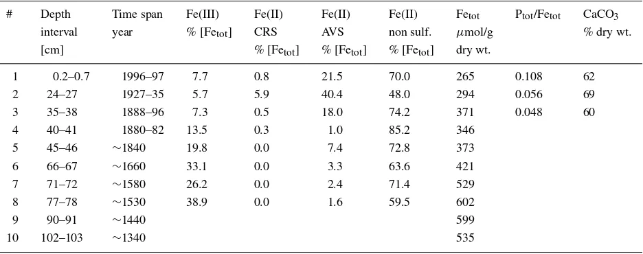
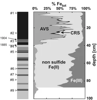
marcasite (Morse et al., 1987). Details are described in Bott (2002). The result-ing Fe speciation profile is given in Figure 1. The Fe(III) content varies from 7.7 mol% Fetot near the sediment-water interface to more than 30% in the oligotrophic section of the core (Table I and Figure 1). CRS represents only a minor component with concentrations below 5.9% in the EXAFS samples (Table I). The important fractions are AVS sulfides and the remaining non-sulfide Fe(II) fraction. AVS con-tributes between 7.3 and 85% to the total Fe fraction (Figure 1) with values for the EXAFS samples ranging from 18 to 40% (Table 1). For the non sulfide Fe(II) fraction minimum and maximum values in the core are 15 and 86% of total Fe, respectively. Total P concentrations are low as compared to total Fe concentrations (less than 11% of total iron, Table I). In the oligotrophic section the AVS fraction is diminished and the non sulfide Fe(II) fraction dominates the speciation. The Fe(III) fraction increases with depth and becomes the second fraction of importance. Thus eutrophic samples have generally low CRS, Fe(III) and phosphate concentrations. As a consequence, iron oxides, pyrite and iron phosphates will be difficult to detect in these samples from the eutrophic lake by EXAFS spectroscopy. By contrast, the Fe(II) sulfides and the undetermined Fe(II) fraction are significant with respect to EXAFS sensitivity. In the oligotrophic section the non sulfide Fe(II) fraction dominates the Fe speciation.
2.3. X-RAY DIFFRACTION ANALYSIS
L
O
R
E
NZ
O
S
P
ADINI
E
T
AL
.
Table I. Chemical analysis and selective extraction of EXAFS samples
# Depth Time span Fe(III) Fe(II) Fe(II) Fe(II) Fetot Ptot/Fetot CaCO3
interval year % [Fetot] CRS AVS non sulf. µmol/g % dry wt.
[cm] % [Fetot] % [Fetot] % [Fetot] dry wt.
1 0.2–0.7 1996–97 7.7 0.8 21.5 70.0 265 0.108 62
2 24–27 1927–35 5.7 5.9 40.4 48.0 294 0.056 69
3 35–38 1888–96 7.3 0.5 18.0 74.2 371 0.048 60
4 40–41 1880–82 13.5 0.3 1.0 85.2 346
5 45–46 ∼1840 19.8 0.0 7.4 72.8 373
6 66–67 ∼1660 33.1 0.0 3.3 63.6 421
7 71–72 ∼1580 26.2 0.0 2.4 71.4 529
8 77–78 ∼1530 38.9 0.0 1.6 59.5 602
9 90–91 ∼1440 599
10 102–103 ∼1340 535
EXAFS OF IRON PHASES IN LAKE SEDIMENTS 5
Figure 1. Schematic stratigraphy of sediment core from the deepest site in Baldeggersee (left). The eutrophic section is represented in black and the oliogotrophic section in light gray. Black line bundles indicate varves in the oligotrophic section. The symbol ‘>’ indicates the sampling locations for the EXAFS analysis. The relative Fe contribution of the AVS, CRS, Fe(II), Fe(III) fractions from selective extraction are given in mole% with respect to total Fe.
chlorite (chlinochlore) and dolomite. Other minerals, noticeably Fe compounds, were not found in the diffraction spectra.
2.4. SAMPLE PREPARATION, EXAFS DATA COLLECTION AND REDUCTION
core sampling in vertical position was achieved by means of an airtight core gate and a core crank. FeK edge EXAFS measurements were performed at the EXAFS D42 station of the L.U.R.E synchrotron radiation facility in Orsay, Paris. Spectra were recorded in fluorescence or transmission mode depending on the metal con-centration. X-ray absorption spectra were treated following a standard procedure (Koningsberger and Prins, 1988). The terminology used here corresponds to that given in Sarret et al. (1998).
2.5. ANALYSIS OF BOND DISTANCES IN IRON MINERALS
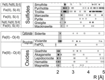
Our analysis of FeK edge EXAFS data from these heterogeneous sediment samples is based on the hypothesis that Fe-carbonates, -phosphates, -sulfides and -oxides may be discriminated according to their Fe-1st shell distances. This working hypo-thesis needs to be verified. The inter-atomic distances of natural reference minerals are thus compared in Figure 2: gray-shaded areas mark the distribution of the Fe-1st shell distances of the given mineral groups. Effectively, the gray box for the Fe-sulfide 1st shell distances reflects the largest distances. Almost all individual Fe-sulfide 1st shell distances are longer than those of other groups. Octahedrally coordinated Fe(II)–S(–II) minerals (smythite, pyrrhotite, troilite) form a distin-guished group of maximum Fe–S bond length as compared to Fe(II)–S(–I) minerals – as is expected from crystal chemical rules. Shortest Fe–S distances are found for tetrahedrally coordinated S atoms (mackinawite, greigite). Compared to Fe-sulfides, Fe(II)–O carbonate and phosphate distances are shorter. The Fe(III)–O group exhibits the shortest bond lengths. Average first shell distances can be de-termined with a precision of≥0.1 Å from EXAFS spectra at the FeK edge. Figure 2 therefore shows that a coarse speciation of the main Fe mineral groups is possible for mineral phases, which have a significant contribution to sediment material.
3. Results and Discussion
3.1. QUALITATIVE SPECTRA ANALYSIS
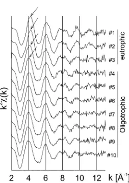
The normalized EXAFS FeK edge k2χ(k) spectra of the sediment samples are
shown in Figure 3. The spectra represent the FeK edge X-ray absorption fine structure of the sediment samples, recorded with increasing wave number, i.e., with increasing energy relative to the FeK edge. The top three samples #1 to #3
relate to the eutrophic lake regime whereas the seven lower samples #4 to #10 come from sediment strata deposited under oligotrophic conditions. Generally all 10 spectra are close in shape. At k < 7 Å−1, thereon referred as low k range,
the signal originates from a single oscillation which relates essentially to the first coordination shell of the central Fe atom. At 8 Å−1 a beating pattern is observed
EXAFS OF IRON PHASES IN LAKE SEDIMENTS 7
Figure 2. Fe-atomic shell distances of minerals considered in the present study. Oxidation states and the mineral groups are given in the left column. The first shell Fe–O and Fe–S distances for each mineral are given in gray. Symbols ∗ and + stand for octahedral and tetrahedral coordination. For the next-nearest shells,△,♦andrefer to Fe, P, S and O neighbors, respectively. Oxygen shells are plotted up to a distance of d(Fe–O) = 3.4 Å.
detail later. In the low k range the top 3 spectra differ nevertheless significantly from the other ones. The raw spectra of the oligotrophic group (#4 to #10) look
almost identical, they have all a k2χ(k) maximum at 4.0 Å−1. By contrast, the
spectra of the eutrophic group (#1 to #3) show this phase maximum slightly shifted towards higher k values (Figure 3, see arrows). This k shift changes continuously from sample #1 to #4. Thus roughly two groups of spectra can be identified: (i) The seven spectra of the oligotrophic section are almost invariant, which indicates a constant speciation with depth. (ii) The three spectra of the eutrophic section change continuously with depth.
Figure 3. k2-weighted EXAFS spectra of sediment samples. Samples #1 to #3 were collected in the eutrophic section, and #4 to #10 in the oligotrophic section.
too low to be discriminated by EXAFS. The signal in the oligotrophic section is therefore certainly dominated by other non-sulfide Fe species.
EXAFS OF IRON PHASES IN LAKE SEDIMENTS 9
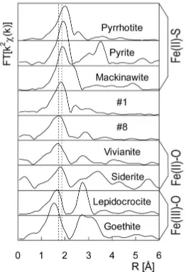
Figure 4. Radial distribution functions (RDFs) of the samples #1 and #8 compared with representative reference compounds.
Figure 4. The positions of the 1st shell maxima of both #1 and #8 compare best to those of vivianite and siderite. Both are Fe(II) minerals with an oxygen lattice. Thus major concentrations of Fe(II)–O minerals are supposed to be present in both samples. In comparison, the 1st peak positions of Fe-sulfides (the Fe(II)–S group) appear at longer distances and the Fe(III)-oxides distances (Fe(III)–O group) are shorter.
of the chemical analysis (Figure 1, Table I). In the eutrophic range two major Fe fractions were detected with specific chemical extraction methods. The first frac-tion consisted of AVS minerals which contribute 22 (#1), 40 (#2) and 18 % (#3), respectively, to the total Fe concentration. This AVS fraction can be related to the Fe(II)–S group contributing to the EXAFS data in Figure 4. The second important fraction could be assigned to non sulfide Fe(II) minerals with contributions of 70 (#1), 48 (#2) and 74 % (#3), respectively, to the total Fe content. This fraction cor-responds to the dominant contribution of the Fe(II)–O group in the RDF of Figure 4. There are two important Fe(II)–O mineral groups: phosphates and carbonates. In general, the total P concentration is too low to bind a significant fraction of the iron in the Fe(II)–O group (Table I). The carbonates are therefore the most likely candidate for iron binding in these sediments.
3.2. QUANTITATIVE SPECTRA ANALYSIS
Statistical analyses of EXAFS data were performed with linear combinations of reference and sample k2
χ(k) spectra and subsequent least square regression
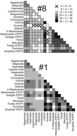
ana-lysis. In a first round a systematic fit procedure was applied: all possible pair combinations of reference spectra (marcasite & siderite, marcasite & goethite etc.) were fitted to the sample spectra #1 and #8, respectively. The results are presented as a two dimensional map of the number of merit in Figure 5. The number of merit represents the sum of least squares between a EXAFS curve calculated as a linear combination of two reference spectra and the measured sample spectra. Crosses on a white background correspond to the best correspondence. The merit of the other squares decreases with increasing darkness.
Oligogrophic section.vivianite itself fits very well to #8, all combinations includ-ing vivianite have correspondinclud-ingly a good merit and most of the best solutions marked with a cross in Figure 5 include this reference mineral. The only com-petitive alternative combines siderite and ferrihydrite. Further linear combinations with good numbers of merit are found when combining two iron oxides, one oxide with siderite or some of the Fe-sulfide references (pyrrhotite, pyrite, troilite). This statistical approach identifies vivianite, siderite, some Fe oxides and Fe sulfides as potential major Fe bearing minerals in the oligotrophic section of the sediment. As already noticed Fe-phosphates are present as a minor fraction only. On the other hand, the best fitting mineral vivianite belongs to the Fe(II)–O group. At this group level the fit result compares well to the speciation scheme expected from RDF findings in the oligotrophic section. Thus, whereas the method fails in correctly predicting the major mineralspeciesthe approach nevertheless results in a valuable proposition for the dominant mineralgroup.
EXAFS OF IRON PHASES IN LAKE SEDIMENTS 11
Figure 5. Map of least-squares sums obtained from the systematic fit procedure for samples #8 and #1. The optimization was achieved by minimizing U, defined as U = (k2χexp −
k2χth)2, whereχexprepresents the observed EXAFS curve, andχthstands for the calculated
is supported by chemical and comparative RDF findings. In particular, the best solution combines mackinawite and vivianite, thus an Fe-sulfide and a Fe(II)– O compound. As for #8, systematic fitting leads to valuable propositions of the dominant mineral groups but fails again in delivering reasonable combinations of mineral species. Vivianite can only represent a minor Fe bearing fraction ac-cording to the chemical analysis results. This species acts as a placeholder for an unknown Fe(II)–O species with similar first shell properties as vivianite. On the other hand, the combined evidence of EXAFS and selective extraction suggests that mackinawite is effectively a major Fe-bearing mineral species.
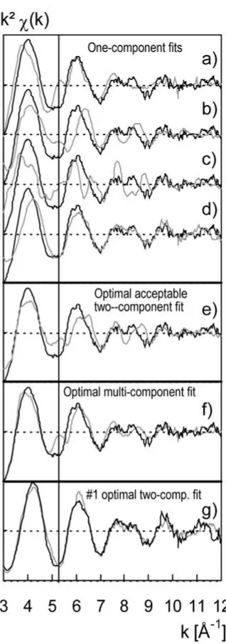
Experimental k2χ(k) spectra were compared in more detail with a selection
of references. Different weights (expressed in %) were given to combinations of reference spectra. The three top fits in Figure 6 compare sample #8 individually to each of the references vivianite, ferrihydrite and siderite. A common systematic deviation between #8 and the three pure references is indicated at 5.3 Å−1 by a
vertical line in Figure 6: the k2χ(k) value of the #8 spectrum is always
signific-antly lower than those of the three reference compounds. It is thus mathematically not possible to solve this misfit by linearly combining the three reference spectra. These fits contrast with the particular fit given in Figure 6d, in which #8 is fitted to #1. This calculation yields the best one-component fit and confirms that the #1 and #8 spectra are very close. No misfit is observed at 5.3 Å−1 and the two
spectra #1 and #8 exhibit both the same beating pattern at 7.7 to 8.3 Å−1. This
similarity suggests that a unique mineral species prevails in both samples #1 and #8 from the eutrophic and oligotrophic section, respectively. To assess this hypothesis fits with 2 and 4 components of sample #8 were performed based on the original reference database excluding the #1 spectrum in the fit procedure. Thus, Figure 6e is a 2-component fit based on siderite and ferrihydrite. Figure 6f represents a 4-component fit with the non-sulfide reference compounds vivianite, siderite, lepidocrocite and ferrihydrate. Both fits 6e and 6f are not satisfying, significant misfits prevail particularly at 5.3 Å. We therefore conclude that the reference data-base is not representative for the speciation in sample #8. Reference spectra of major Fe species are missing, or sample and reference species may have a different local Fe order. The following section is dedicated to the solution of this specific problem.
3.3. PROPOSED SPECIATION
It was already mentioned that all ten samples are close in shape. This fact and in particular the common beating pattern between 7.7 and 8.3 Å−1(Figure 3) are
sec-EXAFS OF IRON PHASES IN LAKE SEDIMENTS 13
tion where it adds to the AVS fraction. To assess this hypothesis a series of fits of the #1 spectrum were performed with the #8. The best two-component fit (Figure 6g) combines the #8 spectrum and that of low crystalline (lc) mackinawite which contributes to the AVS fraction. All other two-component fits excluding the #8 spectra have a significantly lower merit (data not shown).
The next question of interest concerns the mineralogical nature of the #8 spe-cies. Fe replacing Ca in the calcite structure seems to be a valuable proposition to be tested: CO2−3 ligands are abundant in the sediment, calcite and thus also a (Cax, Fe1−x)CO3 solid solution may form (Filippi et al. 1998). In our previous study we found evidence for the formation of (Cax, Mn1−x)CO3(Friedl et al. 1997). An EXAFS spectrum of Fe containing calcite was not available. Therefore a theoretical (Cax, Fe1−x)CO3structure was calculated with the FEFF7 code (Rehr et al. 1991; Zabinsky et al., 1995).
3.4. CALCULATION OF THE(Cax, Fe1−x)CO3STRUCTURE
lepido-EXAFS OF IRON PHASES IN LAKE SEDIMENTS 15
Figure 7. Experimental (black lines) compared to theoretical (grey lines) FeKEXAFS spectra calculatedab initiowith the FEFF7 code. (a) calculated and experimental siderite spectra. (b) same as (a), but the 2nd and 3rd C and O shells are removed in the simulation. (c) the #8 spectrum compared to a calculated siderite FeO6octahedron with a Fe–O distance of 2.144 Å). (d) the #8 spectrum compared to the (Cax, Fe1−x)CO3simulation with the 1st and 4th shells fixed at d(Fe–O) = 2.08 Å and d(Fe–Ca) = 3.94 Å).
crocite and/or ferrihydrate. In the eutrophic section, mackinawite appears as further major species.
4. Conclusions
and linear combination techniques to decipher the Fe speciation in such complex matrices. In our case the method proved successful in deciphering the major Fe species when combined to chemical selective extraction methods. In principle, EX-AFS analysis allowes detecting majorindividualmineral species, whereas specific chemical extraction methods only indicategroupsof minerals such as the AVS and CRS fraction. The two methods are thus complementary. In complex mixtures bulk EXAFS may allow to discriminate solely the dominant species. In particular the linear combination fit approach requires the a priori knowledge of the reference compounds and the associated EXAFS spectra. Thus major species not included in the database may be disregarded. In the given case mackinawite and the (Cax, Fe1−x)CO3solid solution compound could be inferred only by combining EXAFS and chemical analysis results. Also, diagenetic minerals may be more or less sub-stituted and their EXAFS spectra may differ significantly from well-crystallized reference compounds. The validation of EXAFS fits with results from selective extraction is therefore essential.
Acknowledgments
The study was performed within the frame of a bilateral French-Swiss PICS project (No. 310) co-financed by the French CNRS, the French ministry of foreign affairs and the Swiss national science foundation SNF (NF-20-47136.96). The authors gratefully acknowledge the LURE synchrotron facility in Orsay for beamtime.
References
Berner R. A. (1964) Iron sulfides formed from aqueous solutions at low temperatures and atmo-spheric pressure.J. Geol.72, 293–306.
Bott M. (2002) Iron sulfides in Baldeggersee during the last 8000 years: Formation processes, chem-ical speciation and mineralogchem-ical constraints from EXAFS spectroscopy. Ph. D. thesis, ETH, Zürich.
Burdige D. J. (1993) The biogeochemistry of manganese and iron reduction in marine sediments. Earth Science Reviews35, 249–284.
Cornell R. M. and Schwertmann U. (1996) The Iron Oxides. Structure, Properties, Reactions, Occurrence and Uses. VCH Verlagsgesellschaft, Weinheim.
Davison W. (1993) Iron and manganese in lakes.Earth-Science Reviews34, 119–163.
Drodt M., Trautwein A. X., König I., Suess E. and Bender Koch C. (1997) Mössbauer spectroscopic studies on the iron forms of deep-sea sediments.Phys. Chem. Minerals24, 281–293.
Filippi M. L., Lambert P., Hunziker J. C. and Kubler B. (1998) Monitoring of detrial input and resus-pension effects on sediment trap material using mineralogy and stable isotopes (delta O–18 and delta C–13): The case of Lake Neuchatel (Switzerland).Palaeogeogr. Palaeoclim. Palaeoecol.
140, 33–50.
Friedl G., Wehrli B. and Manceau A. (1997) The role of solids in the cycling of manganese in eutrophic lakes – new insights from EXAFS spectroscopy.Geochim. Cosmochim. Acta61, 275– 290.
EXAFS OF IRON PHASES IN LAKE SEDIMENTS 17
Koningsberger D. C. and Prins R. (1988)X-ray Absorption. John Wiley & Sons, New York. Kuno A., Matsuo M. and Numako C. (1999) In situ chemical speciation of iron in estuarine sediments
using XANES spectroscopy with partial least-squares regression.J. Synchrotron Radiation6,
667–669.
Lotter A. F., Sturm M., Teranes J. L. and Wehrli B. (1997) Varve formation since 1885 and high-resolution varve analyses in hypertrophic Baldeggersee (Switzerland).Aquat. Sci.59, 304–325.
Manceau A., Lanson B., Schlegel M. L., Harge J. C., Musso M., Eybert-Berard L., Hazemann J. L., Chateigner D. and Lamble G. (2000) Quantitative Zn speciation in smelter-contaminated soils by EXAFS spectroscopy.Am J. Sci.300, 289–343.
Mettler S., Abdemoula M., Hoehn E., Schoenenberger R., Weidler P. and von Gunten U. (2001) Characterization of iron and manganese precipitates from an in situ ground water treatment plant. Ground Water39, 921–930.
Morse J. W., Millero J. M., Cornwell J. C. and Rickard D. (1987) The chemistry of the Hydrogen Sulfide and Iron Sulfide systems in natural waters.Earth Science Reviews24, 1–42.
Nakano A., Tokonami M. and Morimoto N. (1979) Refinement of 3C pyrrhotite, Fe7S8.Acta Cryst. B35, 722–724.
Nirel P. M. V. and Morel F. M. M. (1990) Pitfalls of sequential extractions.Water Res.24, 1055–1056.
Rehr J. J., Mustre de Leon J., Zabinsky S. I. and Albers R. C. (1991) Theoretical X-ray absorption fine structure standards.J. Am. Chem. Soc.113, 5135–5145.
Sarret G., Manceau A., Spadini L., Roux J.-C., Hazemann J.-L., Soldo Y., Eybert-B,rard L. and Menthonnex J. J. (1998) Structural determination of Zn and Pb binding sites in Penicillium chrysogenum cell wall by EXAFS spectroscopy.Envir. Sci. Technol.32, 1648–1655.
Schaller T., Moor H. C. and Wehrli B. (1997) Sedimentary profiles of Fe, Mn, V, Cr, As and Mo recording signals of changing deep-water oxygen conditions in Baldeggersee.Aquatic Sciences
59, 345–361.
Taillefert M., Lienemann, C.-P., Gaillard J.-F. and Perret D. (2000) Speciation, reactivity, and cycling of Fe and Pb in a meromictic lake.Geochim. Cosmochim. Acta.64, 169–183.
Uda M. (1968) The structure of tetragonal FeS.Zeitschr. Anorg. Allg. Chem.361, 94–98.
Zabinsky S. I., Rehr J. J., Ankudinov A., Albers R. C. and Eller M. J. (1995) Multiple scattering calculations of X-ray absorption spectra.Phys. Rev. B52, 2995–3009.