Conference paper

(1)

SPATIALLY CONSTRAINED GEOSPATIAL DATA CLUSTERING FOR MULTILAYER

SENSOR-BASED MEASUREMENTS

N. M. Dhawale a, _{*, V. I. Adamchuk} a_{, S. O. Prasher} a_{, P. R. L. Dutilleul}b_{, R. B. Ferguson}c

a

Department of Bioresource Engineering, McGill University, Macdonald Campus, Ste-Anne-de-Bellevue, Quebec, H9X 3V9, Canada - nandkishor.dhawale@mail.mcgill.ca

b

Department of Plant Science, McGill University, Macdonald Campus, Ste-Anne-de-Bellevue, Quebec, H9X 3V9, Canada- pierre.dutilleul@mcgill.ca

c

Department of Agronomy and Horticulture, University of Nebraska-Lincoln, Lincoln,

Nebraska, 68508, USA- rferguson1@unl.edu

KEYWORDS: precision agriculture; proximal soil sensing; geospatial data clustering; management zones

ABSTRACT:

One of the most popular approaches to process high-density proximal soil sensing data is to aggregate similar measurements representing unique field conditions. An innovative constraint-based spatial clustering algorithm has been developed. The algorithm seeks to minimize the mean squared error during the interactive grouping of spatially adjacent measurements similar to each other and different from the other parts of the field. After successful implementation of a one soil property scenario, this research was to accommodate multiple layers of soil properties representing the same area under investigation. Six agricultural fields across Nebraska, USA, were chosen to illustrate the algorithm performance. The three layers considered were field elevation and apparent soil electrical conductivity representing both deep and shallow layers of the soil profile. The algorithm was implemented in MATLAB, R2013b. Prior to the process of interactive grouping, geographic coordinates were projected and erroneous data were filtered out. Additional data pre-processing included bringing each data layer to a 20x20 m raster to facilitate multi-layer computations. An interactive grouping starts with a new “nest” search to initiate the first group of measurements that are most different from the rest of the field. This group is grown using a neighbourhood search approach and once growing the group fails to reduce the overall mean squared error, the algorithm seeks to locate a new “nest”, which will grow into another group. This process continues until there is no benefit from separating out an additional part of the field. Results of the six-field trial showed that each case generated a reasonable number of groups which corresponded to agronomic knowledge of the fields. The unique feature of this approach is spatial continuity of each group and capability to process multiple data layers. Further development will involve comparison with a more traditional k-means clustering approach and agronomic model calibration using a targeted soil sampling.

* Corresponding author

1. INTRODUCTION

1.1 General Instructions

While conventional soil sampling techniques are laborious and time consuming, proximal soil sensing (PSS) allows rapid and inexpensive collection of high-density data (Viscarra Rossel and McBratney, 1998; Viscarra Rossel et al., 2010). To pursue various site-specific management practices, spatial data is frequently split into groups (clusters or zones) to represent significantly different growing conditions (Fraise et al., 2001; Ping and Dobermann, 2003). Geo-spatial data clustering is an important process (Li and Wang, 2010), which is widely used in remote sensing (Deng, et. al. 2003), neuroanatomy analysis (Prodanov, et. al, 2007), and other areas. Several different spatial clustering algorithms have been developed to group geospatially dense PSS-based measurements of soil attributes into management zones. For example Management Zone Analyst (Fridgen et al., 2004) represents a publicly available tool accepted by a number of practitioners. The algorithm is based on computing a distance matrix and performing clustering over this new distance matrix. It is closely related to the popular k-means clustering algorithm, where quality of the resulting clusters heavily depends on the selection of initial centroids and the results are not repeatable. However, this method requires

cross-validation to select the best among several runs. (Abdul-Nazeer and Sebastian, 2009). Although the method allows multidimensional data analysis, complexity and frequently occurring discontinuities of management zones make this technology non-robust for potential users (Kerby et al., 2007; Shatar and McBratney, 2001).

Spatial continuity of formed clusters can be achieved by restricting grouping measurements that are not adjacent to each other (Dhawale et al., 2012) through so called Neighbourhood Search Analysis (NSA). This is a form of clustering built on the principle of growing new groups of data points or grid cells with a fixed size through minimization of the mean squared error (MSE). Since previous trials with one measured soil attribute revealed positive outcomes, the objective of this study was to advance an algorithm to allow multiple data layers to be used for delineating spatially constrained groups of high-density soil sensor-based measurements. Field elevation and apparent soil electrical conductivity (ECa) at two depths obtained from six agricultural fields with different levels of spatial structure were used to illustrate the performance of the algorithm developed.

The International Archives of the Photogrammetry, Remote Sensing and Spatial Information Sciences, Volume XL-2, 2014 ISPRS Technical Commission II Symposium, 6 – 8 October 2014, Toronto, Canada

This contribution has been peer-reviewed.

(2)

2. MATERIALS AND METHODS

2.1 Data collection

Six production fields from Nebraska were mapped using Veris 3100 (Veris Technologies, Salina, Kansas, USA) galvanic contact soil ECa mapping unit equipped with an RTK-level, AgGPS 442 (Trimble Navigation Ltd., Sunnyvale, California, USA) and a global navigation satellite system (GNSS) receiver.. The three data layers were: 1) field elevation 2) deep soil ECa (~0-90 cm) obtained with a wide pair of Wanner array electrodes and 3) shallow soil ECa (~0-30 cm) obtained using the narrow pair of electrodes. Table 1 summarises data from the six fields. It has been noted that the two layers of ECa represent similar but not identical spatial patterns, while field elevation does not always correspond to the overall pattern of changing ECa. Therefore, the ideal map of field partitioning would delineate areas with different combinations of the three values significantly different from the average field conditions.

Field ID Area, ha Mean Range SD

Table 1. Summary of data from agricultural fields

2.2 Data pre-processing

All data processing was accomplished using MATLAB R2013b (The MathWorks, Inc. Natick, Massachusetts, USA). To obtain three 2D matrices representing each field, sensor-based data pre-processing involved four steps: 1) removing erroneous data using predefined threshold values of physically feasible measurements, 2) 1D data smoothing using a 5-point moving average technique, 3) projection of local coordinates according to Adamchuk (2001), and 4) 20x20 m averaging of all measurements inside each grid cell. Field elevation data were relative to the lowest grid cell found in every field. The resulting rectangular matrix representing each field covered the entire spatial domain. Grid cells outside field boundaries were assigned zero values. Therefore, no grid cells inside the fields were without corresponding sensor measurements. Smaller grid cell size would also be possible, but require more computation power. The selected resolution using the total of 600-1500 grid cells per field was considered reasonable to reveal field macro-variability.

2.3 Data clustering algorithm

The data clustering algorithm was constructed using an assumption that treating a group of adjacent grid cells separately form the rest of the field would reduce the MSE between individual cell values and the average for corresponding groups:





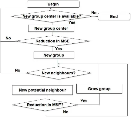
N = the total number of non-zero grid cells

The interactive process of grid cell grouping starts with the assumption that all grid cells belong to the group labelled “1” designated as “the rest of the field”. Grid cells can be grouped together only when they have at least one common side. This assumption is typically referred to as “rook’s rule”. Only nine neighbouring grid cells in a 3x3 configuration can form a new group. The beginning of a new group as well as a merger of a new grid cell to an existing group is accepted when the result produces the lowest MSE. Group enlargement as well as the search for a new group stops when neither action could result in further MSE decrease. Figure 1 illustrates the flowchart of the algorithm developed.

Figure 1. Algorithm flow chart

One minus the ratio of the MSE calculated using equation (1) and the initial MSE (considering that k = 1) indicates the fraction of variability accounted for by the grouping and is equivalent to the coefficient of determination (R2) typically used to quantify the quality of a linear regression model:

1 successfully used for a single data layer. To achieve multilayer analysis, MSE for each data layer should be minimized and R2 maximized. This can be realized by multiplying R2_values.

(3)

Thus, perfect recognition of spatial variability would mean R2 = 1 (measured values within each group are exactly the same), and R2 < 1 once a fraction of the variability is not accounted for. Therefore, the product of three R2 (elevation and two depths of EC) will be small if at least one of the three multipliers is relatively low. Since MSEk=1is a constant value, the same grid cell grouping result will occur when minimizing the product of three MSE estimates as when maximizing the product of three R2 values. Quality partitioning of an agricultural field would occur when R2 for all the data layers would be relatively high with the smallest possible number of identified groups of relatively homogeneous grid cells different from their surroundings. Since the two ECa measurements frequently correlate, the influence of field elevation in this study was made similar to the influence of ECa by raising the elevation R2_{estimate to the second power:}



₂



2

2 2

2

Elevation DeepEC

ShallowEC

Product

R

a a





(3)

Therefore, the algorithm shown in Figure 1 was implemented to maximize product R2 instead of the MSE for a single data layer. No formal statistical analysis and comparison with more traditional spatial clustering techniques were performed at this preliminary stage.

3. RESULTS AND DISCUSSION

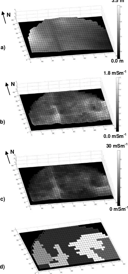
Figure 2 illustrates one of the six fields from the initial trial of the developed algorithm. Areas of the field representing low elevation in the east and high elevation in the west were delineated first with two additional groups emerging later. Figure 3 illustrates that R2 values increased as new groups were formed. Apparently, delineation of groups 2 and 4 were primarily caused by the spatial variability of soil ECa, while groups 3 and 5 emerged predominantly due to differences in field elevation. The algorithm did not locate any new groups of 3x3 grid cells that could further increase the R2 product.

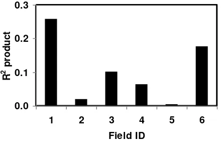
Figure 4 illustrates grid cell grouping for all the fields resulting in a total of 2-8 groups per field. Figure 5 summarises resulting R2 values. The products of these values are shown in Figure 6. Fields 2 and 4 revealed only one group of grid cells that could be separated from the rest of the field while Fields 3 and 4 had 6 and 7 groups, respectively. At the same time, the algorithm produced groups with relatively strong three data layer partitioning for Fields 1, 3, 4, and 6. However, sub-division of Fields 2 and 5 was mainly dominated by field elevation, which resulted in relatively low R2_{products. In both cases, soil EC}

a measurements differed significantly among neighbouring cells, indicating relatively poor spatial structure.

Although the strength of this algorithm is spatial continuity of each group of grid cells, group edges may need smoothing for improved field manageability. Since grid cells poorly associated with their neighbours occur mostly due to field anomalies or erroneous measurements, edge smoothing will always reduce R2 product objective function. The next step in this research will include a comparison of resulting field partitioning with equivalent processing that can be conducted using more traditional k-means-type clustering algorithms (Fraise et al., 2001; Ping and Dobermann, 2003) with suitable pre- and post-processing techniques.

Figure 2. Maps of field elevation (a), shallow ECa (b), deep ECa (c), and delineated groups of grid cells (d) for Field 1.

0.0 0.2 0.4 0.6 0.8 1.0

1 2 3 4 5 Number of grid cell groups

R

2

Product Elevation Deep ECa Shallow ECa

Figure 3. Change in R2 product with number of delineated grid cell groupings.

a)

b)

c)

d) N

N

3.5 m

0.0 m

1.8 mSm-1

0.0 mSm-1

30 mSm-1

0 mSm-1 The International Archives of the Photogrammetry, Remote Sensing and Spatial Information Sciences, Volume XL-2, 2014

ISPRS Technical Commission II Symposium, 6 – 8 October 2014, Toronto, Canada

(4)

Figure 4. Maps of partitioned fields.

0.0 0.2 0.4 0.6 0.8 1.0

1 2 3 4 5 6

Field ID

R

2

Elevation Shallow ECa Deep ECa

Figure 5. R2 values for three data layers used to partition the six experimental fields.

0.0 0.1 0.2 0.3

1 2 3 4 5 6

Field ID

R

2 p

ro

d

u

c

t

Figure 6. R2 products for the six fields.

4. SUMMARY

The spatial clustering algorithm developed in this study is based on a neighbourhood search method and seeks to minimize variance inside each group of interpolated grid pixels corresponding to an unlimited number of sensor-based data layers. Preliminary tests of the algorithm using six production fields illustrated algorithm robustness when delineating field areas with different field elevations and soil ECa measurements. Each spatially constrained group of grid cells with the exception of the first group designated as “the rest of the field” emerged in response to every unique combination of data values relatively constant within each group.

4.1 References

Adamchuk, V.I. 2001. Untangling the GPS String. University of Nebraska Co-operative Extension,EC-01-157, University of Nebraska, Lincoln, Nebraska, USA.

Abdul-Nazeer, K.A., and Sebastian. M. P. 2009. Improving the Accuracy and Efficiency of the K-means Clustering Algorithm. In Proceedings of the World Congress on Engineering, 23(1), pp. 1-3.

Deng, X., Wang, Y., and Peng, H. 2003. The Clustering of High Resolution Remote Sensing Imagery. Journal of Electronics & Information Technology. 25(8), pp. 1073-1080.

Dhawale, N., V. I. Adamchuk, S.O. Prasher, and P.R.L. Dutilleul. 2012. Spatial data clustering using neighbourhood analysis. Paper No. 121337939. St. Joseph, Michigan: ASABE.

Fraisse, C.W., K.A. Sudduth, and N.R. Kitchen. 2001. Delineation of site-specific management zones by unsupervised classification. Trans. ASAE., 44(1), pp. 155-166.

Fridgen, J.J., N.R. Kitchen, K.A. Sudduth, S.T. Drummond, W.J. Wiebold, and C.W. Fraisse. 2004. Management Zone Analyst (MZA): software for subfield management zone delineation. Agron. J., 96, pp. 100-108.

Kerby, A., Marx, D., Samal, A., and Adamchuk, V. 2007. Spatial clustering using the likelihood function. In ICDM Workshops, Seventh IEEE International Conference. pp. 637-642.

Li, Z., and Wang, X. 2010. Spatial Clustering Algorithm Based on Hierarchical-Partition Tree. International Journal of Digital Content Technology and its Applications. 4(6), pp. 26–35.

Ping, J. L., and Dobermann, A. 2003. Creating spatially contiguous yield classes for site-specific management. Agronomy Journal. 95, pp. 1121-1131.

Prodanov, D.P., Nagelkerke, N., and Marani, E. 2007. Spatial clustering analysis in neuroanatomy: Applications of different approaches to motor nerve fiber distribution. Journal of Neuroscience Methods. 160(1), pp. 93-108.

Shatar, T. M., and McBratney, A. 2001. Subdividing a field into contiguous management zones using a k-zones algorithm. In: (Eds.) G. Grenier and S. Blackmore, Proceedings of the 3rd European Conference on Precision Agriculture., Agro-Montpellier ENSAM., France, pp. 115-120.

Viscarra Rossel, R. A., and McBratney, A. B. 1998. Laboratory evaluation of a proximal sensing technique for simultaneous measurement of clay and water content. Geoderma. 85, pp.19-39.

Viscarra Rossel, R. A., McBratney, A. B., and Minasny, B., (Eds.). 2010. Proximal Soil Sensing, Progress in Soil Science Series, Springer-Verlag, New York. New York. USA.

4.2 Acknowledgements

This research was supported in part by funds provided through the National Science and Engineering Research of Canada (NSERC) Discovery Grant; Agricultural Research Division of the University of Nebraska-Lincoln; and Deere and Company. Field 4

Field 1 Field 2

Field 3

Field 5 Field 6