MONITORING SPATIAL PATTERNS OF VEGETATION PHENOLOGY IN
AN AUSTRALIAN TROPICAL TRANSECT USING MODIS EVI
Xuanlong Maa,b
, Alfredo Huetea,⇤, Qiang Yua,b
, Kevin Daviesa
, and Natalia Restrepo Coupea a
Plant Functional Biology and Climate Change Cluster, University of Technology, Sydney, Australia
b
Institute of Geographic Sciences and Natural Resources Research, Chinese Academy of Sciences, Beijing, China
Commission VIII/6
KEY WORDS:NATT, tropical savannas, phenology, climate change, MODIS, EVI
ABSTRACT:
Phenology is receiving increasing interest in the area of climate change and vegetation adaptation to climate. The phenology of a landscape can be used as a key parameter in land surface models and dynamic global vegetation mod-els to more accurately simulate carbon, water and energy exchanges between land cover and atmosphere. However, the characterisation of phenology is lacking in tropical savannas which cover more than 30% of global land area, and are highly vulnerable to climate change. The objective of this study is to investigate the spatial pattern of vegetation phenology along the Northern Australia Tropical Transect (NATT) where the major biomes are wet and dry tropical savannas. For this analysis we used more than 11 years Moderate Resolution Imaging Spectroradiometer (MODIS) Enhanced Vegetation Index (EVI) product from 2000 to 2011. Eight phenological metrics were derived: Start of Sea-son (SOS), End of SeaSea-son (EOS), Length of SeaSea-son (LOS), Maximum EVI (MaxG), Minimum EVI (MinG), annual amplitude (AMP), large integral (LIG), and small integral (SIG) were generated for each year and each pixel. Our results showed there are significant spatial patterns and considerable interannual variations of vegetation phenology along the NATT study area. Generally speaking, vegetation growing season started and ended earlier in the north, and started and ended later in the south, resulting in a southward decrease of growing season length (LOS). Vegetation productivity, which was represented by annual integral EVI (LIG), showed a significant descending trend from the northern part of NATT to the southern part. Segmented regression analysis showed that there exists a distinguishable breakpoint along the latitudinal gradient, at least in terms of annual minimum EVI (EVI), which is located between
18.84◦S to 20.04◦S.
1 INTRODUCTION
Phenology as a subject to study the life cycles of vegeta-tion and the interacvegeta-tions between vegetavegeta-tion and climate (White and Thornton, 1997) is receiving increasing in-terests in global change research. Vegetation phenology can be used as a key parameter in large scale ecosys-tem simulation models (Running and Hunt, 1993) and general circulation models (Sellers et al., 1996). At the same time, vegetation phenology is also an accurate in-dicator of influences by climate change on vegetation growth (Menzel et al., 2006).
Phenological studies of vegetation traditionally utilised ground based techniques (Jeffree, 1960, Sparks and Jef-free, 2000), however, increasing number of studies utilise remote sensing to study vegetation phenology on a large scale (Schwartz, 1999, Zhang et al., 2003, St¨ockli, 2004). Compared with field based cameras or visual inspection, space borne optical sensors such as MERIS (MEdium Resolution Imaging Spectrometer) and MODIS (Mod-erate Resolution Imaging Spectroradiometer) are able to provide daily measurements of variety biophysical and biochemical information of the earth’s surface with moderate spatial resolution.
⇤Corresponding address: Plant functional biology and
cli-mate change cluster, University of Technology, Sydney, PO Box 123, Broadway, NSW, 2000, Australia, Tel: +61 2 9514 4084, Email: [email protected]
However, till now most remote sensing phenology stud-ies focused on temperature and light limited systems (Beurs and Henebry, 2010), with few conducted on wa-ter limited systems (Brown and de Beurs, 2008), and rarely on tropical savannas. Tropical savannas are gen-erally defined as a biome with discrete tree stratum and continuous grassy ground layer (Frost et al., 1986), which covers one-sixth of the global land surface, and con-tributes approximately 30% of the gross primary pro-ductivity (GPP) of all terrestrial ecosystems (House and Hall, 2001). Tropical savannas are also considered par-ticularly vulnerable to climate change (Canadell et al., 2003). Despite the importance of tropical savannas, stud-ies of its vegetation phenology are lacking regardless of the methods, thus restricting our capability to under-stand the impact of possible climate change scenarios on tropical savannas ecosystems.
Previous studies showed that a biogeographical bound-ary existed in the NATT area, which may distributed
around 16-20◦S. 18-20◦S was considered as the south
limit of the influences from monsoonal rainfall
(Bow-man, 1996, Burbidge, 1960), 15-16◦S was considered
as the southern limit of wet season as well as the south-ern limit of monsoon tall-grass savannas (Cook and Heerde-gen, 2001). Meanwhile, in terms of vegetation family
and species, the major changes occur around 16-17◦S
boundary exists, it might be reflected by vegetation phe-nology.
In this study, we mainly focused on two points: 1) using remote sensing to investigate the spatial patterns of veg-etation phenology in the NATT area; 2) try to identify the abrupt change (breakpoint) in terms of the phenolog-ical metrics along the latitude in the NATT, thus provid-ing a phenological perspective on the biogeographical boundary question. Our study showed that there were significant spatial patterns of vegetation phenology in the NATT during past decades, a north-south directional trend was identified. Meanwhile, breakpoint analysis showed that, there was a distinguishable ’breakpoint’
lo-cated around 18◦S to 20◦S,
2 DATA AND METHODS
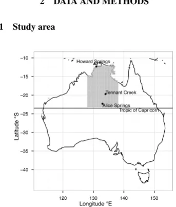
2.1 Study area
Longitude °E
L
a
ti
tu
d
e
°
S
−40 −35 −30 −25 −20 −15 −10
● Howard Springs
● Alice Springs
●Tennant Creek
Tropic of Capricorn
120 130 140 150
Figure 1: The spatial extent of the NATT study area (gray colour area)
This study focussed on Northern Australia Tropical Tran-sect which was extended in this study as a 1.38 million
km2
area which located between latitude 12◦S and 23◦
S and between longitude 128◦E and 138◦E (Fig. 1).
The use of transects has been largely adopted by global change community over past two decades as a standard method to assess spatial patterns of biogeochemical pro-cesses (Koch et al., 1995). The spatial variation of long time constants along the transect can be used as an sur-rogate of predicted temporal variation to understand the future responses to global change (Koch et al., 1995). The Northern Australian Tropical Transect (NATT) was established under IGBP (International Geosphere Bio-sphere Programme) in the mid 1990s, and is one of three transects around world to study global savannas (Koch et al., 1995). Along the NATT, mean annual precipita-tion decreases from nearly 1700mm in the north wet end (Howard Springs) to 300mm in the south dry end (Alice Springs) (Hutley et al., 2011). The vegetation in NATT is a wet-dry savannas gradient where in northern half of NATT, the dominant vegetation is tropical savannas cov-ered by overstory evergreen Eucalyptus and understory annual and perennial C4 grasses (Egan and Williams,
1996). However, in southern half of the NATT the dom-inance of savannas declines, and the domdom-inance of Aca-cia woodlands and shrub lands and hummock grasslands increases. (Bowman and Connors, 1996).
2.2 Data
2.2.1 MOD13C1 EVI A total of more than 11 years
(2000-2011) of MODIS Terra 16-day 0.05◦spatial
reso-lution collection 5 vegetation indices product (MOD13C1) were used in this study. This product is mainly de-signed to provide globally consistent vegetation condi-tions (Running et al., 1994, Justice and Vermote, 1998). In this study, the Enhanced Vegetation Index (EVI) was used as a surrogate for vegetation growth condition. EVI can effectively reduce the soil background and atmo-spheric noise while improving the sensitivity in high biomass regions (Huete et al., 2002). The equation of EVI is:
EVI = 2.5× ρ
nir−ρred
ρnir+ 6×ρred−7.5×ρblue+ 1
(1)
whereρNIR,ρred, andρblueare the wavelengths in the
near infrared, red, and blue bands respectively (Huete et al., 2002).
The residual cloud and aerosol contamination in the orig-inal EVI time series were filtered out based on the qual-ity assurance (QA) flags provided along with the MOD13C1 product.
For pixels without distinct seasonality, such as deserts and water-bodies, no phenology metrics were derived. QA filtered data was temporally gap filled by the av-erage value of the six points before and after the gap. Remaining noise was removed by a Savitzky-Golay fil-ter.
2.3 Methods
2.3.1 Phenological metrics retrieval method In this study, each increase (green-up) and decrease (brown-down) during a growing season was reproduced by two separate four parameters logistic function:
y=a+ b−a 1 +exp(c−t
d )
(2)
where,ais the background EVI before or after growing
season,bis the maximum EVI during growing season,c
is the inflection point when the fitted curve reached the
maximum rising or decreasing speed, dis the scaling
factor which determines the rate of increase or decrease of EVI at inflection point. The parameters were esti-mated based on nonlinear least squares criteria for each pixel and each phenological cycle during 2000-2011, a total of 11 growth cycles.
The phenological transition dates were determined based
on the curvature change rateK0of the fitted curve
whenK0reached first local maximum during the green-up period, and End of Season (EOS) corresponded to
the time whenK0reached last local minima during the
brown-down period. These moments were considered as the transitions of vegetation growing from one lin-ear stage to another (Zhang et al., 2003). The DOY (Day of Year) of SOS and EOS started from July 1 of each year. The length of season was calculated as the difference between SOS and EOS. Other phenological metrics were calculated using function fitted time se-ries. Respectively, Maximum of Greenness (MaxG) and Minimum of Greenness (MinG) were maximum and min-imum EVI values during a phenological cycle; ampli-tude (AMP) was the difference between MaxG and MinG; Large Integral of Greenness (LIG) was the daily inte-grated EVI value for a phenological cycle; Small Inte-gral of Greenness (SIG) was the daily integrated EVI during growing season (defined as a period between SOS and EOS) subtracted daily integrated MinG during the same period.
2.3.2 Segmented regression to identify breakpoints in latitudinal gradients of phenological metrics In this study, segmented linear regression was used to iden-tify the breakpoint for phenological index along the lat-itude. Segmented linear regression applies linear
re-gression to (x, y) data that do not have a linear
rela-tion (Wayne Skaggs, 1996). On the relarela-tions between phenological metrics and latitude, it is hypothesised that there might be a significant breakpoint existed, however, generally the relations do not necessarily have to be lin-ear. So that with segmented linear regression, the break-points can be introduced, among different segments, sep-arate linear regression are applied and by this means nonlinear relations between phenological metrics and latitude might be approximated by a series linear seg-ments (Wayne Skaggs, 1996). By calculation of the con-fidence intervals of breakpoints, optimum breakpoint, which means that the breakpoint with smallest interval can be selected (Oosterbaan et al., 1990).
3 RESULTS AND DISCUSSION
3.1 Spatial patterns of vegetation phenology
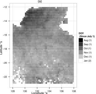
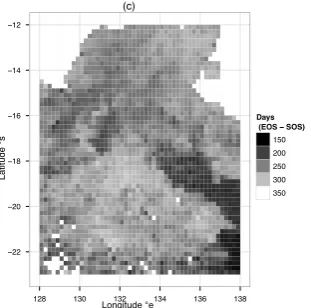
In the NATT study area, all phenological metrics exhib-ited significant spatial patterns in terms of 11 years of average conditions (Fig. 2, 3,4, and 5). Over the NATT, the dates of vegetation growing season onset (SOS) ranged from approximately late August to late January, span-ning a five months time period. While the dates of veg-etation growing season dormancy (EOS) ranged from late February to late October, spanning approximately an eight months time period. The length of vegetation growing season (LOS), which is the difference between EOS and SOS, ranged from about 138 days to 354 days, with differences as large as 216 days (7 months). Ta-ble 1 and TaTa-ble 2 provide detailed statistical summary for all eight phenological metrics over the whole NATT study area.
The latitudinal gradients of vegetation phenology were also very significant in the NATT area. From north to
Table 1: Five-number summary 1 of phenological met-rics in the NATT area. The phenological metmet-rics were the average of 11 years.
SOS EOS LOS MaxG
Minimum 50 243 138 0.1048
25% quantile 120 355 235 0.1794
Median 133 384 258 0.2395
75% quantile 143 414 278 0.2921
Maximum 214 478 354 0.4902
south, the dates of vegetation growing season onset sig-nificantly shifted to later by 3.916 days per latitude de-gree (Fig. 6(a)).While the dates of vegetation growing season dormancy also shifted south to later by approx-imately 1.75 days per latitude degree (Fig. 6(b)), how-ever, the latitudinal trend of EOS was not as strong as the trend of SOS. The trends of SOS and EOS naturally led to the latitudinal trend of LOS (length of season), which showed a southward decreasing by approximately 1.6 days per latitude degree (Fig. 7(a)). The most sig-nificant latitudinal gradient came from LIG (integral of annual EVI), which can be considered as the vegetation annual productivity, showed a almost straight line de-cay, where the latitudinal averaged LIG in the south end of NATT was only approximately 38% of the north end (Fig. 7(b)).
In the temporal scale, the vegetation phenological met-rics in the southern NATT generally had a relatively larger interannual variabilities than the northern NATT (the ver-tical lines in Fig. 6 and 7, which were the temporal stan-dard deviations).
(a)
Longitude °e
L
a
ti
tu
d
e
°
s
−22 −20 −18 −16 −14 −12
128 130 132 134 136 138
DOY (Since July 1)
Aug (1) Sep (1) Oct (1) Nov (1) Dec (1) Jan (2)
Figure 2: Spatial patterns of 11 years (2000-2011) mean SOS (the date of growing season onset) in the NATT.The numbers in the bracket indicate the calendar years, which 1 means first half of phenological year, i.e. from July 1 to December 31, 2 means second half of phenological year, i.e. from next January 1. Original 0.05 degree resolution result had been aggregated to 0.2 degree resolution for plotting purpose.
3.2 Results of breakpoint analysis
The breakpoint analysis showed that at least in terms of annual minimum EVI (MinG), which was considered as a good indicator of tree cover ratio, there was a
(b)
Longitude °e
L
a
ti
tu
d
e
°
s
−22
−20
−18
−16
−14
−12
128 130 132 134 136 138
DOY (Since July 1)
Mar (2) Apr (2) May (2) Jun (2) Jul (2) Aug (2) Sep (2) Oct (2) Nov (2)
Figure 3: Spatial patterns of 11 years (2000-2011) mean EOS (the date of growing season end) in the NATT. The numbers in the bracket indicate the calendar years, which 1 means first half of phenological year, i.e. from July 1 to December 31, 2 means second half of pheno-logical year, i.e. from next January 1. Original 0.05 de-gree resolution result had been aggregated to 0.2 dede-gree resolution for plotting purpose.
(c)
Longitude °e
L
a
ti
tu
d
e
°
s
−22 −20 −18 −16 −14 −12
128 130 132 134 136 138
Days (EOS − SOS)
150
200
250
300
350
Figure 4: Spatial patterns of 11 years (2000-2011) mean LOS (the length of growing season) in the NATT. Origi-nal 0.05 degree resolution result had been aggregated to 0.2 degree resolution for plotting purpose.
and the breakpoint shifted its location inter annually in a approximately 1.18 degree extent (Fig. 8). In the north of this boundary, the annual minimum EVI dropped dra-matically as a function of latitude, however, in the south of this boundary, the downward trend became gradu-ally slowing (Fig. 8). In the south of this boundary, the minimum EVI was generally lower than 0.14, even lower than 0.12 in some year and reached as low as 0.10, which might be considered as soil background. And in the north end, the annual minimum EVI can be as large as 0.24, approximately twofold than its southern coun-terpart (Fig. 8).
4 DISCUSSION AND CONCLUSION
This study has two significances:
(d)
Longitude °e
L
a
ti
tu
d
e
°
s
−22 −20 −18 −16 −14 −12
128 130 132 134 136 138 EVI (Annual integral)
10 40 70 100 130 160 190 220 250
Figure 5: Spatial patterns of 11 years (2000-2011) mean LIG (the annual integral of EVI) in the NATT. Original 0.05 degree resolution result had been aggregated to 0.2 degree resolution for plotting purpose.
Table 2: Five-number summary 2 of phenological met-rics in the NATT area. The phenological metmet-rics were the average of 11 years.
MinG AMP LIG SIG
Minimum 0.0024 0.0053 2.87 2.19
25% quantile 0.1222 0.0519 89.19 55.60
Median 0.1455 0.0824 110.50 75.11
75% quantile 0.1779 0.1182 135.58 91.79
Maximum 0.3458 0.3003 248.74 148.08
a
Latitude (°S)
D
a
te
Oct Nov Dec Jan
● ● ●●●●●●●●
●●●●●●●●●●●●●●● ● ●●●●●●●●●●
●●●●●●●●●●●●●●●●●●●●●●●●●●●●●●●●●●●●●●●●●●● ●●●●●●●●●●●●●●●●●●●●●●●●●●●●●●●●●●●●●●●●●●●●
● ● ● ●●●●●●●●●●●●●●●●●●●●●●
●●●●●●●●●●●●●●●●●●●●●●●●●●●●●●●●●● ●●●●●●●●●●●
●●●●● ●●●●
●●● ● ●● ●●●●
● ● ●●●●
● ●
SOS=62.992+3.916×Latitude R2=0.8503
12 14 16 18 20 22
b
Latitude (°S)
D
a
te
May Jun Jul Aug Sep
●● ●●●●●●●●
●● ● ● ●●●●●●●●●●●●●●●●
●●●●●●●●●●●● ●●●●●●●●●●●●●●●●●●●●●●●●●●●●●●●
● ●●●●●●●●●●●●●●●●●●●●●●
●●●●●●●●●● ●●●●●●●●●●●●●●●
●●●●● ●●●●
●● ●●●●●●●
●●●●●● ●● ● ●● ●●●●●●
● ● ● ●●●●
●● ● ●● ●●●●●●●●●
●●● ●●●
●●●●●●●●●●●●●● ● ● ●●●
● ●●●●
●● ● ● ● ● ● ●●● ● ●●
EOS=351.2527+1.7456×Latitude R2=
0.138
12 14 16 18 20 22
Figure 6: Latitudinal gradients of vegetation phenol-ogy along the transect (a) SOS; (b) EOS. The equations show the phenological metrics as a function of latitude. The vertical lines are the temporal standard deviations of these latitudinal gradients.
1. To our knowledge, this study was the first inves-tigation of vegetation phenology using an almost an complete MODIS datasets for the NATT study area.
a LOS=279.4381−1.6362×Latitude
R2=0.1402 LIG=279.6161−9.4874×Latitude
R2 =0.9713
12 14 16 18 20 22
Figure 7: Latitudinal gradients of vegetation phenol-ogy along the transect (a) LOS; (b) LIG. The equations show the phenological metrics as a function of latitude. The vertical lines are the temporal standard deviations of these latitudinal gradients.
Latitude
Figure 8: Spatial distributions and interannual variation of MinG breakpoints. Small points are interannual vari-ations of annual minimum EVI along the latitude, large points are interannual variations of breakpoints. The north and south boundaries of these breakpoints are in-dicated by two vertical lines. The numbers give the ac-tual latitudes of north and south boundary.
From an evolutionary point of view, the vegetation phe-nology is the result of biological adaption to historical climate. However, it is hard to study the variations of vegetation phenology in the time dimension over a short period. The assumption of using sub-continental scale transects to study global change problems is that the spa-tial variation can be used as a surrogate of the temporal variations (Koch et al., 1995). So that even if it is dif-ficult to predict vegetation phenology in future, we do have the possibilities to derive the vegetation phenology under different climate change scenarios through the in-vestigation in the spatial dimensions, which is more fea-sible (Cook and Heerdegen, 2001).
The southward decreasing trends of vegetation produc-tivity (annual integral EVI) can be attributed to both in-ternal and exin-ternal factors. Inin-ternally, tree species rich-ness are decreasing southward along NATT (Williams et al., 1996). Previous studies suggested that decreasing of woody richness always associates with decreasing of vegetation productivity (Waring et al., 2006, MacArthur, 1969). Externally, environmental factors , including
pre-cipitation and soil water content, also have significant north-south decreasing trend in this area (Williams et al., 1996).
In the temporal scale, large interannual variations of veg-etation phenology may suggest that the environmental factors, which control vegetation growth, should have corresponding interannual variations in this area. In the NATT, both precipitation amount and precipitation pat-tern have significant interannual variations (Cook and Heerdegen, 2001).
In this study we used annual minimum EVI, which is considered as an indicator of evergreen component, to investigate the spatial distribution of a biogeographical boundary in the NATT area. However, in addition to annual minimum EVI, we still have seven other pheno-logical metrics available. This study suggested the po-tential to define the biogeographical boundary from a vegetation phenology perspective. Future research will attempt to identify this boundary using other phenolog-ical metrics.
In conclusion, this study characterized eight vegetation phenological metrics for a sub-continental tropical tran-sect spanning the past 11 years. Our results showed that these metrics had significant spatial patterns as well as considerable interannual variations. However, the en-vironmental control on these phenological patterns re-mains unclear, which requiring further investigations with the collaboration efforts from both remote sensing and climatological perspectives.
ACKNOWLEDGEMENTS
This research was partially support by ARC-(DP1115479) grant entitled “Integrating remote sensing, landscape flux measurements, and phenology to understand the impacts of climate change on Australian landscapes” (Huete, CI). The first author appreciates the financial support from Chinese Scholarship Council, which enables the first au-thor to study abroad and focus on his research.
REFERENCES
Beurs, K. M. D. and Henebry, G. M., 2010. Spatio-Temporal Statisticall Methods for Modelling Land Sur-face Phenology. Springer Netherlands, Dordrecht.
Bowman, D., 1996. Diversity Patterns of Woody
Species on a Latitudinal Transect From the Monsoon Tropics to Desert in the Northern Territory, Australia. Australian Journal of Botany 44(5), pp. 571–580.
Bowman, D. M. J. S. and Connors, G. T., 1996. Does low temperature cause the dominance of Acacia on the central Australian mountains? Evidence from a latitu-dinal gradient from 11o to 26o South in the Northern
Territory, Australia. Journal of Biogeography 23(2),
pp. 245–256.
Burbidge, N., 1960. The phytogeography of the
aus-tralian region. Australian Journal of Botany 8(2),
pp. 75–211.
Canadell, J. G., Dickinson, R., Hibbard, K., Raupach, M., Apps, M., Chedin, A., Chen, C.-T. A., Cox, P. M., Druffel, E. R. M., Field, C., Lankao, P. R., Lebell, L., Patwardhan, A., Sabine, C., Valentini, R., Yamagata, Y. and Young, O., 2003. Global Carbon Project The Science Framework and Implementation. Technical Re-port 1.
Cook, G. D. and Heerdegen, R. G., 2001. Spatial vari-ation in the durvari-ation of the rainy season in monsoonal Australia. International Journal of Climatology 21(14), pp. 1723–1732.
Egan, J. L. and Williams, R. J., 1996. Lifeform distribu-tions of woodland plant species along a moisture avail-ability gradient in Australia’s monsoonal tropics. Aust. Systematic Bot. 9(2), pp. 205–217.
Frost, P., Medina, E., Menaut, J.-C., Solbrig, O., Swift,
M. and Walker, B., 1986. Responses of savannas
to stress and disturbance: A proposal for collabrative programme of research. Biology International special is(10), pp. 81.
House, J. I. and Hall, D. O., 2001. Productivity of Trop-ical Savannas and Grasslands. Terrestrial Global Pro-ductivity (16), pp. 363–400.
Huete, A., Didan, K., Miura, T., Rodriguez, E. P., Gao, X. and Ferreira, L. G., 2002. Overview of the radiomet-ric and biophysical performance of the MODIS vegeta-tion indices. Remote Sensing of Environment 83(1-2), pp. 195–213.
Hutley, L. B., BERINGER, J., Isaac, P. R., Hacker, J. M. and Cernusak, L. A., 2011. A sub-continental scale liv-ing laboratory: Spatial patterns of savanna vegetation over a rainfall gradient in northern Australia. Agricul-tural and Forest Meteorology pp. 1–12.
Jeffree, E. P., 1960. Some long-term means from the phenological reports (1891-1948) of the Royal Meteo-rological Society. Quarterly Journal of the Royal Mete-orological Society 86(367), pp. 95–103.
Justice, C. O. and Vermote, E., 1998. The Moderate Resolution Imaging Spectroradiometer (MODIS): Land remote sensing for global change research. Geoscience and . . . .
Koch, G. W., Vitousek, P. M., Steffen, W. L. and Walker, B. H., 1995. Terrestrial transects for global change re-search. Vegetatio 121(1-2), pp. 53–65.
MacArthur, R. H., 1969. Patterns of communities in the tropics. Biological Journal of the Linnean Society 1(2), pp. 19–30.
Menzel, A., Sparks, T. H., Estrella, N., Koch, E., Aasa, A., Ahas, R., Alm-K¨ubler, K., Bissolli, P., Braslavsk´a, O., Briede, A., Chmielewski, F. M., Crepinsek, Z., Cur-nel, Y., Dahl, A. s., Defila, C., Donnelly, A., Filella, Y., Jatczak, K., M˚a ge, F., Mestre, A., Nordli, O. y., Pe˜nuelas, J., Pirinen, P., Remiˇsov´a, V., Scheifinger, H., Striz, M., Susnik, A., Van Vliet, A. J. H., Wielgolaski, F.-E., Zach, S. and Zust, A., 2006. European pheno-logical response to climate change matches the warming pattern. Global Change Biology 12(10), pp. 1969–1976.
Oosterbaan, R., Sharma, D., Singh, K. and Rao, K.,
1990. Crop production and soil salinity: evaluation
of field data from India by segmented linear regression with breakpoint. Proceedings of the symposium on land drainage for salinity control in arid and semiarid regions 3, pp. 1–12.
Running, S. W. and Hunt, E. R., 1993. Generalization of a forest ecosystem process model for other biomes, BIOME-BGC, and an application for global-scale mod-els. In: J. R. Ehleringer and C. B. Field (eds), Scaling physiological processes leaf to globe, Academic Press, chapter 8, pp. 141–158.
Running, S. W., Justice, C. O., Salomonson, V., Hall, D., Barker, J., Kaufmann, Y. J., Strahler, A. H., Huete, A. R., Muller, J. P., Vanderbilt, V., Wan, Z. M., Teillet, P. and Carneggie, D., 1994. Terrestrial remote sensing science and algorithms planned for EOS/MODIS. Inter-national Journal of Remote Sensing 15(17), pp. 3587– 3620.
Schwartz, M. D., 1999. Surface phenology and satellite sensor-derived onset of greenness: an initial compari-son. International Journal of Remote Sensing.
Sellers, P. J., Randall, D. A., Collatz, G. J., Berry, J. A., Field, C. B., Dazlich, D. A., Zhang, C., Collelo, G. D. and Bounoua, L., 1996. A revised land surface parame-terization (SiB2) for atmospheric GCMs .1. Model for-mulation. Journal of Climate 9(4), pp. 676–705.
Sparks, T. H. and Jeffree, E. P., 2000. An examination of the relationship between flowering times and temper-ature at the national scale using long-term phenological records from the UK. International Journal of . . . .
St¨ockli, R., 2004. European plant phenology and cli-mate as seen in a 20-year AVHRR land-surface parame-ter dataset. Inparame-ternational Journal of Remote Sensing.
Waring, R. H., Milner, K. S., Jolly, W. M., Phillips, L. and McWethy, D., 2006. Assessment of site index and forest growth capacity across the Pacific and Inland Northwest U.S.A. with a MODIS satellite-derived vege-tation index. Forest Ecology and Management 228(1-3), pp. 285–291.
Wayne Skaggs, R., 1996. Drainage principles and
applications. Agricultural Water Management 31(3),
pp. 307–309.
White, M. A. and Thornton, P. E., 1997. A continental phenology model for monitoring vegetation responses to interannual climatic variability. Global . . . .
Williams, R. J., Duff, G. A., Bowman, D. M. J. S. and Cook, G. D., 1996. Variation in the composition and structure of tropical savannas as a function of rainfall and soil texture along a large-scale climatic gradient in the Northern Territory, Australia. Journal of Biogeogra-phy 23(6), pp. 747–756.