Volume 25, Number 2, 2010, 143 – 154
INDUSTRIALIZATION AND DE-INDUSTRIALIZATION IN
INDONESIA 1983-2008: A KALDORIAN APPROACH
D.S. Priyarsono
Bogor Agricultural University (priyarsono@yahoo.com)
Titi Kanti Lestari
Statistics Indonesia (tekael61@yahoo.com)
Diah Ananta Dewi
Statistics Indonesia (a_diahdewi@yahoo.com )
Abstract
Economists have for a long time discussed the causes of economic growth and the mechanisms behind it. Kaldor viewed advanced economies as having a dual nature very similar to that of developing countries, with an agricultural sector with low productivity and surplus labour, and a capital intensive industrial sector characterized by rapid technical change and increasing returns. The transfer of labour resources from the agricultural sector to the industrial sector depends on the growth of the latter’s derived demand for labour. With this background this study attempts to show the periods when the Indonesian economy indicated the processes of industrialization and deindustrialization. It also attempts to identify whether the economy experienced positive deindustrialization (i.e., showed signs of economic maturity where service sector substituted the role of industrial sector as the engine of growth) or negative deindustrialization (i.e., showed signs of economic stagnancy where industrial sector could not grow rapidly enough to absorb surplus labour from agricultural sector). Lastly, this study attemps to analyze several factors that might be responsible for the process of the deindustrialization.
Keywords: industrialization, deindustrialization, economic growth
INTRODUCTION
Kaldor’s hypothesis that manufacturing is the engine of economic growth in a region (Kaldor, 1966) was constructed based on his-torical data of developed as well as developing countries. One important lesson that can be learned from economic history of developed countries is that the countries experienced high economic growth when the dominant role of
share of primary sectors, increasing percentage of urban population, and increasing share of added value of manufacturing in the GDP.
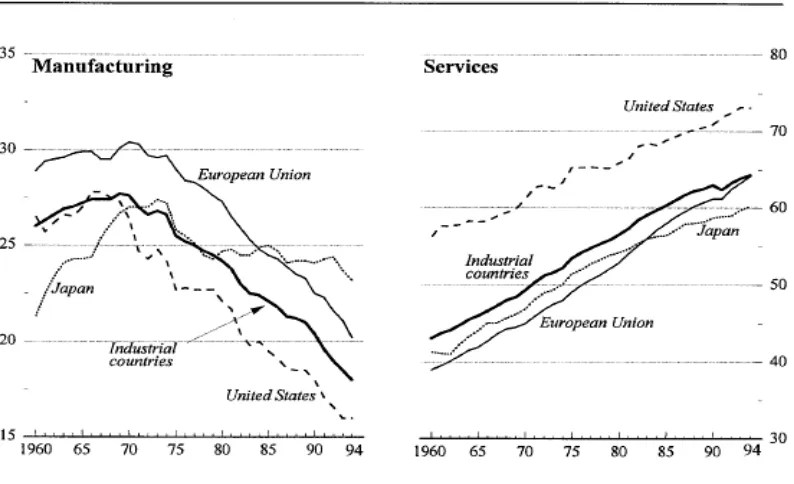
After reaching a certain level of industri-alization (sometimes called a mature level of industrialization), many developed countries experienced the process of de-industrialization which is characterized by decreasing contribu-tion of manufacturing sectors and increasing contribution of service sectors to the total employment as well as total GDP of the economies (Rowthorn & Wells, 1987). Figure 1 illustrates these phenomena.
De-industrialization occurs because of various factors including changes in interna-tional specialization pattern and decreasing of competitive advantage of manufacturing sector in an economy (Kuncoro, 2007).
Not all developing economies follow the industrialization-deindustrialization path ex-perienced by the developed countries. Some of them experience de-industrialization before they reached the mature level of industrializa-tion. This premature or abnormal phenomenon is sometimes called negative de-industrializa-tion (Kitson & Michie, 1997). It is character-ized by low trade balance, productivity, na-tional income, and life standard of the society in the economy.
This study attempts to analysese the role of manufacturing sector in Indonesia during the era of industrialization as well as de-industrialization. It also attempts to identify whether the de-industrialization in Indonesia is negative or positive. Finally, it identifies factors that are responsible for the process of de-industrialization in Indonesia.
Source: IMF (1997)
LITERATURE REVIEW
Kaldor’s Law. According to Kaldor’s First Law, manufacturing is the engine of growth in an economy. This hypothesis can be expressed as a regression equation
q = a1 + b1m (1)
where q is total growth of output and m is growth of manufacturing sector. To increase the power of test of the hypothesis, Kaldor proposed two additional regression equations (Felipe, 1998):
q = a2 + b2 (m - nm) (2)
nm = a3 + b3 m (3)
Equation (2) states that the greater the difference between the growth of manufactur-ing sector (m) and the growth of non-manufacturing sector (nm) the greater the growth of output (q). The growth of non-manufacturing sector depends on the growth of manufacturing sector. With statistically significant positive parameters of b1, b2, and
b3, these three equations sufficiently show that
manufacturing is the engine of growth in an economy.
The positive correlation between q and m can be explained by the fact that the high growth of output in manufacturing sector pulls labours from sectors that have lower produc-tivity. This process of transfer leads to a higher productivity in all sectors, and therefore it leads to a higher productivity of the whole economy which means a higher economic growth. This transfer process is sometimes called economic transition from an immature level to an intermediate level of economic development.
Manufacturing sector normally has strong backward and forward linkages. It pulls its upstream sectors by using their outputs as its input. Furthermore, its output is used as one of important inputs in the production process in the downstream sectors. This fact explains a statistically significant positive parameter b3 in
Equation (3).
The Kaldor’s Second Law which is also called Kaldor-Verdoorn Law states that labour productivity in manufacturing sector is posi-tively correlated with growth of output in the sector. Following Knell (2004), the law can be described in the following three equations.
q = p + e (4)
p = a4 + b4q (5)
e = a5 + b5q (6)
In these equations p and e are, respec-tively, growth of labour productivity and growth of labour in manufacturing sector.
The Kaldor’s Third Law states that pro-ductivity of non-manufacturing sector is positively correlated with growth of output of manufacturing sector.
Industrialization and De-industrializa-tion. Industrialization can be perceived as a structural change from agriculture-dominant to manufacture-dominant economy. Several theo-ries and models have attempted to explain the process of industrialization (see for example, Gollin et al, 2002). Empirical analysis of structural transformation for the case of Indonesian economy was reported by Kuncoro (2007).
Singh (1977), IMF (1997, 1998), Felipe (1998), Jalilian and Weiss (2000), Rowthorn and Coutts (2004), Dasgupta and Singh (2005, 2006), Suwarman (2006), and Libanio et al (2007).
METHODOLOGY
The Hypotheses. This study tests the following hypotheses, (1) manufacturing sec-tor is the engine of growth in the Indonesian economy, (2) Indonesia is experiencing negative de-industrialization, and (3) there are several factors that significantly affect the process of de-industrialization in Indonesia.
The data. To test the hypotheses, secon-dary data from various publications of Statistics Indonesia (Badan Pusat Statistik) were utilized. They are generally quarterly time series data covering the years of 1983-2008. Price related data were standardized so that all were measured using year of 2000 price. Some data that are not quarterly were interpolated using cubic spline method. See Gerald & Wheatley (1994) for a technical discussion on this method.
The econometric modelling. A stationar-ity test is applied to each variable. If at least one variable involved is not stationary, error correction model or vector error correction model (ECM/VECM) is utilized. ECM/VECM can identify short-run and long-run relations among the variables analyzed. However, if all variables are stationary, ordinary linear regres-sion analysis is sufficient (Enders, 2004).
THE ROLE OF MANUFACTURING SEC-TOR IN THE INDONESIAN ECONOMY
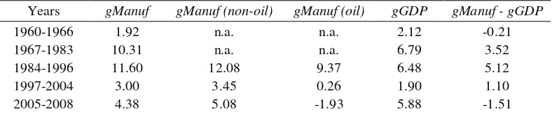
To start exploring the process of indus-trialization and de-indusindus-trialization, the data of growth of manufacturing sector were com-pared to the data of growth of GDP in the Indonesian economy for the period of 1960-2008 (see Table 1). The Indonesian economic development can be perceived as being started more or less officially after the political development relatively settled down in early 1960s. As can be seen in the table, in the first years of the development (1960-1966) the growth of manufacturing sector (1.92%) was less than that of the whole economy (2.12%).
During the first three Soeharto Admini-stration’s Five Year Development Plans (Repelita I-III, 1967-1983), economic devel-opment was focused on the primary sectors. In the manufacturing sector, chemical related industries were developed, such as fertilizers, cement, pulp, and paper. The oil boom that was characterized by high oil price and high domestic production of oil helped boosting theGDP economic growth during this period. Consistent with Kaldor’s First Law, Dasgupta and Singh (2006) states that the higher the difference between growth of manufacturing sector and growth of GDP, the higher the growth of GDP. Data of the 1967-1983 period and the previous period are in line with this statement.
Table 1. Growth of Manufacturing Sector and Gross Domestic Product 1960-2008 (%)
Years gManuf gManuf (non-oil) gManuf (oil) gGDP gManuf - gGDP n.a. = not available, gManuf = growth of manufacturing sector, gGDP = growth of GDP
From Repelita IV to the advent of the global financial crisis (1984-1996), oil price decreased. The government started to put higher priority on non-oil manufacturing sector. The average growth of manufacturing sector during this period increased to 11.6%. The very rapid growth of this sector was not proportionately accompanied by the growth of capacity to supply the raw material for manufacturing sector. Consequently, import of the raw materials increased during this period. The higher difference between the growth of manufacturing company and the growth of the GDP did not lead to higher average of GDP growth. The difference between gManuf and gGDP in the period of 1967-1983 and 1984-1996 are 3.52% and 5.12%, respectively. Meanwhile, the gGDP growths during the two periods are 6.79% and 6.48%, respectively. This indicates that the high growth of manufacturing sector during the previous period was a result of the oil booming instead of a result of maturity of the industrial structure.
During 1997-2004 the Indonesian econ-omy experienced financial crisis and its recovery. The positive average growth of GDP (1.90%) was maintained because of, among other things, the growth of non-oil manufac-turing sectors. In the following period (2005-2008) the growth of GDP was relatively high (5.88%). However, its difference from the
growth of manufacturing sector was negative (minus 1.51%). This indicates that the source of growth was not manufacturing sector but, instead, it was transportation and telecom-munication sector.
To confirm the conclusion from the previous data exploration, the Kaldorian approach was applied. The stationarity test showed that all of the involved variables were stationary. Therefore simple linear regression analysis could be utilized using the data of 1983-2008 as follow (Equations 7-9).
All of the regression equations give low coefficients of determination (R2) which may indicate that more explaining variables need to be included into the equations in order for the models to be able to better explain the variation of the dependent variables. However, the fact that in Equation (7) the coefficients are statistically significantly different from zero does support Kaldor’s First Law. Thus, it can be concluded that during the years manufacturing sector was the engine of growth of the economy. It should be noted, however, that this conclusion is sensitive to the selected period of time. Using time period of 1967-1992 Felipe (1998) found a different conclusion, stating that Kaldor’s Law did not prevail in the Indonesian economy. Dasril (1993) found that the role of manufacturing sector as the engine of growth was more significant in years after 1980.
Equations 7-9
gGDP = 0.67* + 0.33** gManuf (7) t-Stat = (1.77) (4.98) F-Stat = 24.85 R2 = 0.20
p-Val = (0.0790) (0.0000) (0.0000) DW = 2.3969
gGDP = 1.46** – 0.19** (gManuf – gNonManuf) (8) t-Stat = (3.84) (–3.14) F-Stat = 9.89 R2 = 0.09
p-Val = (0.0002) (0.0022) (0.0022) DW = 2.3937
gNonManuf = 0.92* + 0.14* gManuf (9)
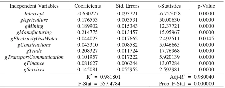
The negative coefficient in Equation (8) does not follow Kaldor’s Law. Probably non-manufacturing sectors such as agriculture and trade did significantly contribute to the GDP of the economy during the observed years. To identify contribution of sectoral growths to the total economic growth, a linear regression analysis was applied (see Table 2). The regres-sion coefficient of growth of manufacturing sector (gManufacturing, 0.214775) is approxi-mately equal to that of trading sector (gTrade, 0.208327). This indicates that the growth of both sectors have approximately the same effects on the growth of added value.
Equation (9) supports Kaldor’s First Law, i.e. a one percent increase in growth of
manu-facturing sector would increase the growth of non-manufacturing sector by 0.14 percent. This is because the growth of output in manufacturing sector leads to a transfer of labour from less productive sectors to more productive ones. This process would result in productivity increase in all sectors. The facts that manufacturing sector has strong backward and forward linkages, as previously men-tioned, confirm further the Kaldor’s First Law. Kaldor’s Second and Third Laws were tested using the following regression equa-tions. Equation (10) confirms the law that labour productivity depends significantly on growth of GDP, i.e. the higher the growth of GDP the higher the labour productivity.
gProductivity = –0.55 + 0.99 gGDP (10)
Table 2. Regression Analysis: Growth of GDP (Dependent) and Its Factors (Sectoral Growths) 1983-2008
Equations (11) and (12) do not show statistically significant coefficients. No impli-cations can be discussed from these regression equations.
Equation (13) supports further Kaldor’s Law. It can be concluded then that manu-facturing is (one of) the engine(s) of economic growth also applies to the Indonesian economy. The fact that growth of trade also contributes equally significantly to the growth of added value needs a further analysis on the relation between this variable and the growth of manufacturing sector. The following regres-sion equation supports further the Kaldor’s Law.
gTrade= 0.95 + 0.28 gManuf (14)
t-Stat = (1.75) (2.96) F-Stat = 8.73 R2 = 0.08
p-Val=(0.0835) (0.0039) (0.0039) DW = 2.1997
THE PROCESS OF DE-INDUSTRIALI-ZATION IN INDONESIA
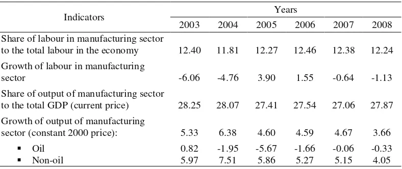
A quick observation on recent economic data (2003-2008) leads to fairly strong indication that the Indonesian economy is experiencing the process of
de-industrializa-tion (see Table 3). The share of manufacturing labour to the total labour is stagnant, nevertheless it shows signs of declining. The average growth of labour in manufacturing sector is negative. The growth of the sector’s output is positive, but its share to the econ-omy’s output is declining. These indicators show indeed the process of de-industrializa-tion, but at the same time there is also a sign of slowdown in the growth of the whole economy (see Table 3). In conclusion, the on-going process can be categorized as negative de-industrialization.
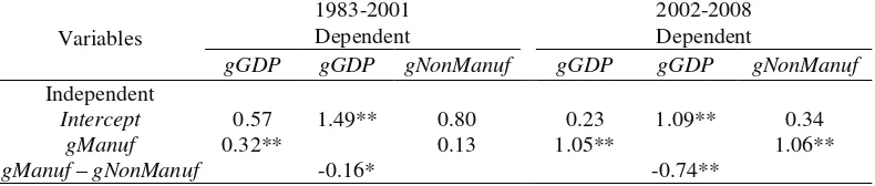
It is interesting to test the Kaldor’s First Law in the Indonesian economy during the industrialization period (1983-2001) as well as the de-industrialization period (2001-2008). Table 4 shows the results of regression analy-ses. In both periods, it is evident that manu-facturing sector was the engine of growth in the economy (see the significant coefficients of gManuf when the dependent variable is gGDP). During the industrialization period and the de-industrialization period, the coefficients of gManuf when the dependent variable is gGDP are 0.32 and 1.05, and both are significant at α = 0.01.
Table 3. Some Indicators of De-industrialization Process in the Indonesian Economy (%)
Indicators Years
2003 2004 2005 2006 2007 2008 Share of labour in manufacturing sector
to the total labour in the economy Growth of labour in manufacturing sector
Share of output of manufacturing sector to the total GDP (current price)
Growth of output of manufacturing sector (constant 2000 price):
Table 4. Evaluation of the Kaldor’s First Law on Two Time Periods: Coefficients of the Simple Regression Equations
Variables
1983-2001 2002-2008
Dependent Dependent
gGDP gGDP gNonManuf gGDP gGDP gNonManuf
Independent Intercept
gManuf gManuf – gNonManuf
0.57 0.32**
1.49**
-0.16*
0.80 0.13
0.23 1.05**
1.09**
-0.74**
0.34 1.06**
*significant at α=5%, **significant at α=1%
A closer look at the coefficients may lead to a conclusion that the dependence of the economy on manufacturing sector is getting stronger (the coefficient increases from 0.32 to 1.05). Therefore it is unfortunate that several indicators show declining performance of manufacturing sector recently, such as (1) decreasing number of units of manufacturing firms, (2) decreasing competitiveness of manufacturing industries, (3) slowdown in the rate of new investments in manufacturing sector, (4) decreasing bank credits for manu-facturing sector, and (5) decreasing consump-tion of electricity by manufacturing sector. Basri (2009) has discussed this.
FACTORS OF DE-INDUSTRIALIZA-TION IN INDONESIA
Following IMF (1997, 1998), Rowthorn and Coutts (2004), and Dasgupta and Singh (2006), an econometric model was established for analyzing the factors that affect the process of de-industrialization in Indonesia as follow.
EmpShare = α0 + α1 ln(Y) + α2 (ln(Y))2 +
α3 I + Σi>3 αi Zi (15)
The dependent variable (share of labour in manufacturing sector to the total labour in the economy) is a proxy of the concept of industrialization. Y and I stand for, respec-tively, per capita income, (approximated by per capita GDP) and investment (approxi-mated by gross fixed capital forming as percentage of GDP). Z represents other
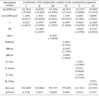
variables such as TB (trade balance = export – import), Open (openness = export + import), MModal (imported capital), MBaku (imported raw material), MKons (imported consumer good), X_USA (export to the USA), X_Japan (export to Japan), X_Sing (export to Singa-pore), and M_China (import from China). All of these variables are measured in percentages relative to the GDP. Testing for stationarity was conducted to each variable involved in the econometric model. The result of the test leads to the use of co-integration and vector error correction model as the method of the analy-sis. Table 5 exhibits the result of the econo-metric analysis.
From Table 5 it can be inferred that there is a positive relationship between per capita income and share of employment in manu-facturing sector. This fact is in line with the well known Engel’s Law1 where an increase of per capita income would lead to an increase in demand for manufactured products. In turn, it would increase the share of employment in manufacturing sector.
The table also implies that a decrease in investment would lead to a decrease in the employment share in manufacturing sector which in turn leads to the process of de-industrialization. In this case, investment often means expenditure for manufacturing prod-ucts. Thus, investment means not only as input
1 Ernst Engel (1821-1896) is German statistician and
economist. For a brief discussion on the applications of
for but also output of production in manu-facturing sector.
Trade balance is defined as difference be-tween export and import. It represents con-sumer’s taste toward exported and imported manufacturing products. A decrease in trade balance would decrease employment share in manufacturing sector. Conversely, an increase in trade balance would increase employment share in the sector. This characteristic is repre-sented in equations II, V, and VI.
This table is the output of data processing using Eviews 6.0. Negative signs (minus)
indicate positive relationship. Conversely, positive signs (plus) indicate negative relation-ship. Numbers in the parentheses are values of the t-Statistics.
Openness is represented by the sum of export and import. Equation III in the Table shows that openness has a positive relationship with employment share in manufacturing sector. Competitiveness of domestic product in international markets will determine the demand for the product. Prescriptions for increasing competitiveness have long been discussed in the public discourse but it has Table 5. Coefficients of the Cointegration Equations with EmpShare as the Dependent Variable
Independent variable
Coefficients of the independent variables in the cointegration equations
I II III IV V VI
ln(GDPCap) -42.4932 [-10.496]
-43.9782 [-10.604]
-19.4764 [-4.4382]
-45.3937 [-12.543]
-19.2374 [-6.0060]
-28.7965 [-4.1915] (ln (GDPCap))2 1.2499
[9.6817]
1.3835 [10.4078]
0.8818 [8.4631]
1.1555 [10.9522]
0.6587 [6.3983]
0.8059 [3.2651]
I -0.2827
[-4.4837]
-0.4787 [-4.5594]
0.0795 [1.3053]
-0.4597 [-8.5966]
-0.3654 [-5.6524]
-0.4269 [-3.8975]
TB -0.2460
[-1.8397]
-0.5622 [-6.5594]
-0.1227 [-0.8830]
Open -0.1842
[-5.4639]
MModal 2.4603
[4.7519]
MBaku -0.1957
[-2.1544]
MKons 1.0288
[7.5079]
X_USA -1.7071
[-6.2404]
X_Japan 0.9321
[9.9040]
X_Sing 1.9794
[5.7145]
M_China 2.5933
[2.5716] Intercept 330.8605 335.4662 99.2739 379.4485 131.5143 233.1914
been very difficult to implement them. Among the prescriptions are reforming financial market systems, improving public services, ensuring the rules of law in labour markets, and improving market economic efficiency through anti-trust regulations.
An increase in imported capital as well as consumer’s goods pushes the process of de-industrialization. Some imported capital sub-stitute labour in manufacturing sector. In addition, imported consumer goods also sub-stitute domestic demand for output of manu-facturing sector. The impact of increasing trend of flooding of Chinese products in domestic markets as a result of the implemen-tation of ASEAN China Free Trade Agree-ment can easily be predicted. Conversely, exports to major countries like Japan, Singapore, and the USA prevent the process of de-industrialization. Unfortunately, increase of export rate to these countries has not been reported.
CONCLUSIONS
Manufacturing sector has been an engine of growth in the Indonesian economy during the industrialization as well as de-industriali-zation era. The process of de-industrialide-industriali-zation in Indonesia tends to be negative. This result was found based on Caldaria approach. Analysis in the section on Factors of De-industrialization in Indonesia led to a conclusion that the negative de-industrializa-tion was not a “natural phenomenon” that followed experience of developed countries. Instead, it was a result of shocks such as low rate of investments, low rate of trade balance, increasing rate of imports of capital as well as consumer goods which would be facilitated further by the recent implementation interna-tional trade agreement.
The rate of de-industrialization should be reduced by improving competiveness of domestic products, boosting new investments, and increasing labour productivity. Many prescriptions for public policies have been
formulated; none of them, however, is easy to implement.
Further study can be suggested in two directions. Firstly, it is interesting to analysese any correlation between process of industri-alization (or de-industriindustri-alization) and types of government (authoritarian, democratic, or others). It is fairly obvious that a consistent industrial policy can be implemented only by a strong government. Secondly, it is important to approach the topic with different methodol-ogy. While valid and robust, error correction model is not the sole econometric model that is capable of attacking the problem. Other models, for example simultaneous equations models, are justifiably possible to be used as instruments for testing Kaldor’s hypotheses.
ACKNOWLEDGEMENTS
Earlier versions of this paper were presented in an academic seminar in Bogor Agricultural University (February 6, 2010) and in Interna-tional Conference on Business and Economics in Bukittinggi, West Sumatera (April 16, 2010). The authors gratefully acknowledge the financial support from the Statistics Indonesia (Badan Pusat Statistik) for this research. Any errors that may remain are solely the authors’ responsibility. For correspondence, contact priyarsono@yahoo.com.
SOURCES OF THE DATA
Variable Name Source
gPDB Directorate of Production Accounts, BPS-Statistics Indonesia
gManuf Directorate of Production Accounts, BPS-Statistics Indonesia
gNonManuf Directorate of Production Accounts, BPS-Statistics Indonesia
Population Statistics, BPS-Statistics Indonesia gEmp Directorate of Population
Statistics, BPS-Statistics Indonesia
gPNonManuf Directorate of Production Accounts and Directorate of Population Statistics, BPS-Statistics Indonesia EmpShare Directorate of Population
Statistics, BPS-Statistics Indonesia
OutShare Directorate of Production Accounts, BPS-Statistics Indonesia
PDBCap Directorate of Production Accounts, BPS-Statistics Indonesia
I Directorate of Production Accounts, BPS-Statistics Indonesia
TB Indikator Ekonomi (Economic
Indicators) 1983-2008, published monthly, BPS-Statistics Indonesia
Open Indikator Ekonomi (Economic Indicators) 1983-2008, published monthly, BPS-Statistics Indonesia
MModal Indikator Ekonomi (Economic Indicators) 1983-2008, published monthly, BPS-Statistics Indonesia
MBaku Indicator Ekonomi (Economic Indicators) 1983-2008, published monthly, BPS-Statistics Indonesia
MKons Indikator Ekonomi (Economic Indicators) 1983-2008, published monthly, BPS-Statistics Indonesia
X_USA Indikator Ekonomi (Economic Indicators) 1983-2008, published monthly, BPS-Statistics Indonesia
X_Japan Indikator Ekonomi (Economic Indicators) 1983-2008, published monthly, BPS-Statistics Indonesia
X_Sing Indikator Ekonomi (Economic Indicators) 1983-2008, published monthly, BPS-Statistics Indonesia
M_China Indikator Ekonomi (Economic Indicators) 1983-2008, published monthly, BPS-Statistics Indonesia
REFERENCES
Basri, F., 2009. “Deindustrialisasi” [De-industrialization]. Tempo Weekly News Magazine, 30 November - 5 December 2009, 102 – 103.
Dasgupta, S. and A. Singh, 2005. ‘Will Ser-vices be the New Engine of Indian Economic Growth?’. Journal of Develop-ment and Change. Vol. 36: 1035-1057. Dasgupta, S. and A. Singh, 2006.
“Manufacturing, Services and Premature Deindustrialization in Developing Countries: A Kaldorian Analysis”, Research Paper No. 2006/49. United Nations University.
Dasril, A.S.N., 1993. “Pertumbuhan dan Pe-rubahan Struktur Produksi Sektor Perta-nian dalam Industrialisasi di Indonesia, 1971 – 1990” [Growth and Change in Production Structure of Agriculture Sector in Industrialization in Indonesia, 1971-1990], Dissertation, Bogor Agricultural University.
Enders, W., 2004. Applied Econometrics: Time Series Analysis. John Wiley and Sons. New York.
Gerald, C. and P. Wheatley, 1994. Applied Numerical Analysis. Addison-Wesley, Reading, Massachusetts.
International Monetary Fund [IMF]. 1997. “Deindustrialization: Causes and Implica-tions”, IMF Working Paper.
International Monetary Fund [IMF]. 1998. “Growth, Trade, and Deindustrialization”, IMF Working Paper.
Jalilian, H. and J. Weiss, 2000. ‘De-industri-alization in Sub-Saharan: Myth or Crisis’. Journal of American Economics. Vol. 9, No. 1:24-43.
Kaldor, N., 1966. Causes of the Slow Rate of Economic Growth of the United Kingdom: an Inaugural Lecture. Cambridge: Cambridge University Press.
Kuncoro, M., 2007. Ekonomika Industri Indo-nesia [Industrial Economics of Indonesian Economy]. Penerbit Andi, Yogyakarta. Kitson, M. and J. Michie, 1997. “Does
Manu-facturing Matter?” Management Research News, Vol. 20, No. 2/3: 63.
Knell, M., 2004. ‘Structural Change and The Kaldor-Verdoorn Law in the 1990s’. Revue
D’Economie Industrielle No. 105, 1st trimester.
Libanio, G. and S. Moro, 2007. Manufacturing Industry and Economic Growth in Latin America: A Kaldorian Approach. http://www.networkideas.org/ ideasact/ Jun07/ ia19_Beijing_Conference.htm Rowthorn, R. and K. Coutts, 2004.
‘De-indus-trialization and the Balance of Payments in Advanced Economies’. Cambridge Journal of Economics, Vol. 28: 767-790. Ruky, I.M.S., 2008. “Industrialisasi di
Indone-sia: Dalam Jebakan Mekanisme Pasar dan Desentralisasi” [Industrialization in Indo-nesia: In the Trap of Market Mechanism and Decentralization], Inaugural Speech for Professorship in Faculty of Economics, University of Indonesia. Jakarta: UI. Singh, A., 1977. ‘UK Industry and the World
Economy: A Case of De-industrialization?’. Cambridge Journal of Economics, Vol. 1, No. 2: 113-136. Suwarman, W., 2006. “Faktor-faktor yang
Mendorong Terjadinya Proses Deindustri-alisasi di Indonesi” [Factors that Push the Process of Industrialization in Indonesia], Thesis. University of Indonesia.