T H E J O U R N A L O F H U M A N R E S O U R C E S • 47 • 1
Month of Birth and Children’s
Health in India
Michael Lokshin
Sergiy Radyakin
A B S T R A C T
We use data from three waves of India National Family Health Survey to explore the relationship between the month of birth and the health out-comes of young children in India. We find that children born during the monsoon months have lower anthropometric scores compared to children born during the fall-winter months. We propose and test hypotheses that could explain such a correlation. Our results emphasize the importance of seasonal variations in environmental conditions at the time of birth in de-termining health outcomes of young children in India. Policy interventions that affect these conditions could effectively impact the health and achieve-ments of these children, in a manner similar to nutrition and micronutrient supplementation programs.
I. Introduction
A large literature in economics, human biology, and medicine has been devoted to understanding the effects of early childhood conditions on outcomes later in life (see, for example, Alderman, Hoddinott and Kinsey 2001 and 2006; Martorell 1999; Beaton 1993). Research has consistently shown that the month of birth is an important predictor of health outcomes, morbidity, and mortality. But, so far, no convincing theories have been proposed to explain this association.
Most of the studies showing correlations between the month of birth and children’s health outcomes have been restricted to high-income settings. The correlation be-tween an individual’s height and his/her month or season of birth was documented by Weber et al. (1998), for Australia; Kihlbom and Johansson (2004) for Sweden;
Michael Lokshin, mlokshin@worldbank.org, and, Sergiy Radyakin, sradyaking@worldbank.org, are both at the Development Research Group, World Bank, 1818 H Street NW, Washington, D.C., 20433. Authors thank Harold Alderman, Jishnu Das, Monica Das Gupta, Toan Q. Do, and Mark Villa for their con-structive comments. The findings, interpretations, and conclusions of this paper are those of the authors and should not be attributed to the World Bank, its Executive Directors, or the countries they represent. The data used in this article can be obtained beginning June 2012 through May 2015 from the authors. [Submitted May 2009; accepted March 2011]
Lokshin and Radyakin 175
Shephard et al.(1979) and Koscinski et al.(2004) for Poland. Early exposure to cold conditions was reported to be associated with higher weight during adulthood in England (Phillips and Young 2000). Van Hanswijck de Jonge et al.(2003), using data from the United States, found that birth weight and early infancy weight gains varied by season and were modified by ethnicity. Tanaka et al. (2007) showed that in Japan the height and weight of schoolchildren were influenced by their months and seasons of birth.
In this paper we use data from three rounds of the India National Family Health Survey (NFHS) to (i) quantify the effect of the month of birth on children’s anthro-pometrics, and (ii) test the hypotheses that might explain the relationship between the months of birth and children’s health outcomes. We find that Indian children born during the monsoon months have worse health outcomes than children born during fall-winter months. The “month-of-birth” effect is shown to be present in all three waves of the NFHS and persists after controlling for a wide set of observable and unobservable characteristics. The effect is large: The differences in height among children born during the monsoons and other children are comparable to the differ-ences in health outcomes between children born to illiterate mothers and to mothers with completed primary education.
The empirical tests conclude that one of the likely explanations for the observed pattern of changes in children’s health by the month of birth could be a higher prevalence of malnutrition and a wider exposure to diseases in the lean monsoon season. Our results show that seasonal climatic variations affect the environmental conditions at the time of birth and determine health outcomes for young children in India. Policy interventions that influence such conditions might be as effective in improving children’s health as nutrition and micronutrient supplementation programs and could drive long-term economic growth by leading to healthier and more pro-ductive adults.1
This paper contributes to the research on child health and nutrition in several ways. First, in contrast to the existing medical literature on the effect of the month of birth on individual health, we try to present a comprehensive causal analysis of this phenomenon, taking into account both socio-economic and environmental fac-tors that might affect children’s health outcomes. Second, we analyze the impact of the months of birth on children’s health in a context of a poor developing country, as compared to most of the literature on this topic, which focuses on developed countries. Third, we demonstrate the “month-of-birth” effect for children younger than three years of age; the majority of studies analyze the consequences of season-ality of birth on outcomes in adult life. Our results prove to be useful in allowing for greater precision in the use of climatic data as explanatory variables in an analysis of health outcomes.
The following section describes the setting of our data and shows some descriptive results. Section III sets up the main question of the paper. Section IV outlines and tests the main hypotheses explaining the association between the month of birth and
176 The Journal of Human Resources
children’s health outcomes. Section V discusses policy implications and offers some conclusions.
II. Data and Descriptive Statistics
This analysis uses data from three waves of the India NFHS (1992/ 1993, 1998/1999, and 2005/2006). The NFHS is a survey of representative house-holds covering states and territories of India containing approximately 99 percent of its population. The survey structure corresponds to the typical structure of demo-graphic and health surveys (DHS) conducted in several other countries. Our main sample contains information on 45,279 children from the 1992/1993 round; 30,984 children from 1998/1999 round; and 48,679 children from 2005/2006 round of the India NFHS.2These children were residing correspondingly in 33,032, 26,056, and 33,968 households.
The NFHS uses three types of questionnaires: The household questionnaire col-lects information on the family structure and background, and on various character-istics of household members. The woman’s questionnaire is administered to women aged 15 to 49 and covers dates and survival status of all births, current pregnancy status, childbearing intentions, and childcare practices. The village questionnaire gathers information on the village area and population.We use the constructed house-hold wealth index as a measure of househouse-hold welfare. The descriptive statistics for the main variables used in this paper are shown in Table 1.
We focused our analysis on the age-adjusted measure of height-for-age (HAZ), which reflects children’s development relative to a reference population of well-nourished children (World Health Organization 2006).3The height-for-age (stunting) is an indicator of the long-term effect of malnutrition (Dibley et al. 1987). For comparability between the rounds of NFHS, we restricted our sample to children less than 36 months of age.
Malnutrition is highly prevalent in India. According to NFHS data, about 80 percent of children under the age of three were underweight in 1992, with minimal changes in 1998 and 2005. In 1992, 72 percent of boys and 70 percent of girls were stunted.4The proportion of stunted children had decreased to 65 percent by 2005. The overall averages of HAZ rose over the years for both boys and girls. The average
2. The number of observations in the 1998/1999 round is smaller because NFHS-2 collected height and weight information only for the last two children, under three years of age, of ever-married women who were interviewed.
3. The analysis of relation of month of birth and weight-for-age (WAZ) z-scores is presented in a working paper version of this paper (Lokshin and Radyakin 2009). Across rounds of NFHS, about 10 percent of eligible children were not measured, either because the children were not at home, or because their mothers refused to allow the measurements (Lokshin, Das Gupta, and Ivaschenko 2005). We find no relationship between this attrition and the seasonality of birth, gender, or type of the family (results are available from authors).
Lokshin and Radyakin 177
HAZ had risen for boys from ⳮ1.9 in 1992 toⳮ1.5 in 2005. Girls experienced
similar improvements in health outcomes between 1992 and 2005.
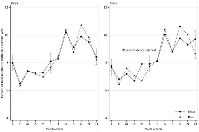
The distributions of births by calendar months by gender and for urban and rural samples are presented in Figure 1.5The proportions of boys and girls born in each month are similar. The highest birth rates are registered in August, September, and October—these children were conceived in winter. The fewest children were born during the winter months of December, January and February—these children were conceived in spring. The wedding season in India, which falls in the months from November to February could partially explain this seasonality of birth (Medora 2003). Figure 2 shows the proportion of children, among all children born in a particular month, who died before the age of three years. The incidence of mortality appears to be unrelated to the month of birth of boys and girls.
In addition to the data from NFHS, we use historical rainfall data from TS2.1 database supported by the Tyndall Centre for Climate Change Research at University of East Anglia in Norwich, U. K. This database contains monthly meteorological data for the period from 1901 to 2002 at the nodes of a global grid spaced at 0.25 degree latitude and longitude width (Mitchell and Jones 2005). We assigned the monthly rainfall data to the districts of NFHS covered in 1992 and 1998 rounds. The effect of the rainfall on children’s health is identified through the variation in the rainfall over the three years for which we observe children in each round of NFHS.
III. Variations of child health outcomes by month of
birth
Figure 3 shows the changes in height-for-ageZⳮscores by the month
of birth for boys and girls in the pooled sample of three rounds of NFHS.6 Anthro-pometric measures appeared to be the lowest for children born in summer and im-proving for children born in fall and early winter. This relationship held for both girls and boys. For example, if the average HAZ for boys born in urban areas of India in June was about ⳮ1.61 (standard error of 0.05), HAZ for boys born in
December wasⳮ1.17 (SE 0.06). The average HAZ increased fromⳮ1.78 for girls
born in urban areas in June toⳮ1.21 for girls born in December.
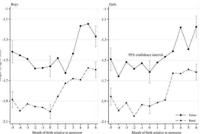
Figure 4 shows the average HAZ by months-of-birth normalized to the beginning of the monsoon season that starts in late May/early June in the southern states of India and in late July in Northern India. According to this normalization, children born in June in the southern states of India would have a normalized month-of-birth
5. The results shown in Figure 1 are calculated based on the sample of children younger than 36 months of age ever born in the household. The distribution of birth by month constructed based on the sample of survived children is similar to one shown in Figure 1.
178
The
Journal
of
Human
Resources
Table 1
Descriptive Statistics for the Main Explanatory Variables.*
Urban Rural
Boys Girls Boys Girls
Mean
Standard
Error Mean
Standard
Error Mean
Standard
Error Mean
Standard Error
Survey year dummies
1992 0.282 0.004 0.274 0.004 0.312 0.003 0.300 0.003 1998 0.317 0.005 0.321 0.004 0.379 0.003 0.389 0.003 2005 0.401 0.005 0.405 0.005 0.310 0.003 0.311 0.003 Child’s current age (in months) 17.84 0.100 18.02 0.096 17.26 0.067 17.44 0.065 Birth order
First-born 0.360 0.005 0.344 0.005 0.279 0.003 0.275 0.003 Second-born 0.302 0.005 0.311 0.004 0.252 0.003 0.249 0.003 Third-born 0.157 0.004 0.162 0.004 0.176 0.003 0.179 0.002 Fourth-born 0.083 0.003 0.086 0.003 0.112 0.002 0.113 0.002 Fifth-born 0.045 0.002 0.044 0.002 0.073 0.002 0.075 0.002 Sixth-born 0.026 0.002 0.024 0.001 0.047 0.001 0.048 0.001 Seventh-born 0.013 0.001 0.014 0.001 0.026 0.001 0.029 0.001 Eighth-born 0.015 0.001 0.016 0.001 0.034 0.001 0.032 0.001 Mother’s current age (in years) months) 26.35 0.049 26.52 0.047 26.08 0.037 26.12 0.035 Education of the mother (years) (in years) 6.693 0.053 6.892 0.050 3.196 0.028 3.280 0.027 Education of the mother (categories)
Lokshin
and
Radyakin
179
Incomplete secondary 0.307 0.005 0.318 0.004 0.193 0.003 0.201 0.003 Complete secondary 0.085 0.003 0.094 0.003 0.038 0.001 0.041 0.001 Higher 0.163 0.004 0.167 0.004 0.032 0.001 0.033 0.001 Scheduled caste 0.143 0.003 0.150 0.003 0.174 0.003 0.180 0.002 Scheduled tribe 0.087 0.003 0.083 0.003 0.175 0.003 0.165 0.002 Religion
Hindu religion 0.684 0.005 0.696 0.004 0.752 0.003 0.751 0.003 Muslim religion 0.196 0.004 0.178 0.004 0.114 0.002 0.119 0.002 Christian religion 0.082 0.003 0.080 0.003 0.083 0.002 0.076 0.002 Sikh religion 0.017 0.001 0.022 0.001 0.029 0.001 0.030 0.001 Other or no religion 0.021 0.001 0.024 0.001 0.023 0.001 0.023 0.001 Wealth index score 0.605 0.009 0.642 0.009 0.488 0.005 0.462 0.005 Urban 7.005 0.035 6.980 0.033 7.598 0.025 7.614 0.024 Household size 0.326 0.001 0.324 0.001 0.331 0.001 0.329 0.001 Share of children 0–6 years 0.094 0.001 0.095 0.001 0.123 0.001 0.124 0.001 Share of children 7–14 years 0.266 0.001 0.267 0.001 0.238 0.001 0.238 0.001 Share of adult males 0.266 0.001 0.267 0.001 0.238 0.001 0.238 0.001 Share of adult females 0.029 0.001 0.029 0.001 0.035 0.000 0.037 0.000 Share of elderly 0.657 0.005 0.667 0.004 0.127 0.002 0.133 0.002 Type of toilet
Flush toilet 0.139 0.003 0.139 0.003 0.128 0.002 0.123 0.002 Latrine 0.204 0.004 0.194 0.004 0.745 0.003 0.744 0.003 Other or none 0.685 0.005 0.685 0.004 0.246 0.003 0.249 0.003 Source of drinking water
Piped water 0.270 0.004 0.265 0.004 0.654 0.003 0.658 0.003 Well or hand pump 0.028 0.002 0.029 0.002 0.087 0.002 0.079 0.002 Surface, river, rain, etc 0.016 0.001 0.020 0.001 0.013 0.001 0.013 0.001
Number of observations 10,099 11,038 22,756 24,358
180 The Journal of Human Resources
Figure 1
Percent of Total Number of Births by Month of Birth
of 0, and children born in November would have a normalized month-of-birth equal to six. The trends in health outcomes depicted in Figure 4 are similar to those of Figure 3: Children born during the monsoon months are more likely to be stunted than the children born during the six months after the start of the monsoon.7
Would the effect of the month of birth on a child’s health be significant after controlling for the characteristics of a household, a mother, and a child? To find the answer to this question we rely on a standard theoretical framework of household utility maximization that incorporates the production function determining child’s health (Behrman and Deolalikar 1988). According to that theory, a household utility is a function of consumption and leisure of household members, as well as the quality (health) and quantity of their children. A household maximizes its utility subject to standard budget constraints and the restrictions imposed by the health production function. The household demand for childi’s healthZidepends on a set
of exogenous characteristics of a childXi, household characteristicsXh,
character-istics of its motherXm, community characteristicsXc, and some unobserved factors
Lokshin and Radyakin 181
Figure 2
Proportion of Children that Died Before the Age of 36 Months Among All Children Born in a Particular Month
captured by random error εi (Thomas, Strauss, and Henriques 1991). This relation can be expressed as:
Z⳱Z(X,X ,X,X,ε).
(1) i i i m h c i
The child’s characteristics include, among others, its month of birth. In the linearized form, the production function of child’s health (Equation 1) can be expressed as:
11 ¯
Z⳱XⳭ ␣M Ⳮε,
(2) i i
兺
k ik ik⳱1
182 The Journal of Human Resources
Figure 3
Health Outcomes (HAZ) by Month of Birth and Gender
The coefficients on the control variables in the regressions used in Table 2 reveal the expected relationship between child health outcomes and the characteristics of a household, a mother and a child. A higher birth order has a negative impact on the health outcomes for both boys and girls (for example, Horton 1988; Angrist and Evans 1998). Consistent with the findings in the literature (for example, Holmes 2006) health outcomes deteriorate with the age of a child. Children living in wealth-ier households and with better-educated mothers are less likely to be stunted. The relationship between a child’s health and his/her mother’s age has an inverted U-shape: HAZ improves with the mother’s age till the age of about 40 and then declines for children of older mothers.
The potential endogeneity of the month-of-birth could have strong implications for the findings of this paper. Suppose parents believe that children born during certain months of the year are more likely to get sick. Then parents would try to plan their pregnancies to give birth in months most favorable for their children’s health. Or, parents might try to compensate the perceived negative effects by pro-viding better care for children born in “bad” months. In the presence of an unob-served heterogeneity in the parental inputs to the production function of a child’s health, the variation in health outcomes by the month of birth could be partially attributed to differences in the parental behavior (for example, Rosenzweig and Shultz 1982).
Lokshin and Radyakin 183
Figure 4
Health outcomes (HAZ) by gender and the month of birth normalized relative to the beginning of monsoon season
heterogeneity in parental inputs to the production function of children’s health. j
can be correlated with the month in which a child is born. Then, Equation 2 will have a following form:
11
¯
Z ⳱X Ⳮ ␣ M Ⳮ( Ⳮ) s.t. Corr(M ,)⳱0; Corr(M ,)⬆0.
(3) ij ij
兺
k ijk ij j ijk j ijk jk⳱1
Under the assumption that the unobserved heterogeneity in parental inputs (for ex-ample, far-sightedness of the parents) is constant over time (siblings), we can account for the endogeneity of the month-of-birth by estimating the fixed-effect (FE) re-gression on the sample of siblings, thus removing the household-specific component
j. The household FE would also absorb a host of other time-invariant geographical
differences that might affect child health outcomes. This regression includes explan-atory variables that differ among the siblings living in the same household: dummies for the month of birth, age of a child and the child’s birth order. The bottom panel of Table 2 shows that most of the FE coefficients on the 11 dummies for the months of birth are statistically significant.8The seasonal patterns in child health are similar to patterns revealed by OLS estimations: children born in fall-winter months are healthier compared to children born in summer.
184
The
Journal
of
Human
Resources
Table 2
Does child’s Height-for-age Z-score Depend on the Month of birth? (Regression on the Pooled Sample of Three rounds of NFHS. Coefficients on the month-of-birth dummies).
Urban Rural
Boys Girls Boys Girls
Coefficient
Standard
Error Coefficient
Standard
Error Coefficient
Standard
Error Coefficient
Standard Error
Calendar month
January ⳮ0.281*** 0.069 ⳮ0.102 0.072 ⳮ0.315*** 0.049 ⳮ0.317*** 0.052 February ⳮ0.328*** 0.072 ⳮ0.363*** 0.074 ⳮ0.388*** 0.052 ⳮ0.429*** 0.054 March ⳮ0.339*** 0.070 ⳮ0.399*** 0.071 ⳮ0.486*** 0.049 ⳮ0.448*** 0.051 April ⳮ0.535*** 0.069 ⳮ0.338*** 0.075 ⳮ0.426*** 0.050 ⳮ0.564*** 0.053 May ⳮ0.507*** 0.070 ⳮ0.312*** 0.071 ⳮ0.528*** 0.050 ⳮ0.536*** 0.054 June ⳮ0.490*** 0.068 ⳮ0.523*** 0.070 ⳮ0.494*** 0.049 ⳮ0.531*** 0.051 July ⳮ0.383*** 0.067 ⳮ0.245*** 0.070 ⳮ0.422*** 0.047 ⳮ0.527*** 0.050 August ⳮ0.455*** 0.063 ⳮ0.270*** 0.066 ⳮ0.313*** 0.045 ⳮ0.374*** 0.047 September ⳮ0.357*** 0.065 ⳮ0.242*** 0.068 ⳮ0.233*** 0.047 ⳮ0.270*** 0.050 October ⳮ0.111* 0.065 ⳮ0.088 0.066 ⳮ0.182*** 0.045 ⳮ0.151*** 0.047 November ⳮ0.117* 0.065 ⳮ0.027 0.067 ⳮ0.030 0.046⽤ ⳮ0.170*** 0.048 December Reference month
Number of observations 11,027 10,098 24,357 22,751
R2 0.167 0.190 0.155 0.176
Month relative to monsoon
Lokshin
and
Radyakin
185
ⳮ2 ⳮ0.328*** 0.071 ⳮ0.423*** 0.075 ⳮ0.380*** 0.050 ⳮ0.424*** 0.054 ⳮ1 ⳮ0.372*** 0.070 ⳮ0.323*** 0.072 ⳮ0.372*** 0.049 ⳮ0.332*** 0.052 Monsoon starts ⳮ0.264*** 0.068 ⳮ0.401*** 0.070 ⳮ0.402*** 0.048 ⳮ0.350*** 0.051 Ⳮ1 ⳮ0.206*** 0.067 ⳮ0.301*** 0.069 ⳮ0.270*** 0.047 ⳮ0.301*** 0.050 Ⳮ2 ⳮ0.331*** 0.065 ⳮ0.330*** 0.068 ⳮ0.154*** 0.047 ⳮ0.237*** 0.049 Ⳮ3 ⳮ0.178*** 0.066 ⳮ0.228*** 0.068 ⳮ0.099** 0.047 0.002 0.049 Ⳮ4 0.091 0.066 ⳮ0.024 0.068 ⳮ0.101** 0.046 ⳮ0.021 0.048 Ⳮ5 0.140** 0.067⽤ ⳮ0.138** 0.068 0.055 0.047 ⳮ0.000 0.050 6 months after monsoon Reference month
Number of observations 11,027 10,098 24,357 22,751
R2 0.166 0.189 0.153 0.174
Month relative to monsoon: FE
5 months prior to monsoon ⳮ0.758** 0.295 ⳮ0.836*** 0.287 ⳮ0.346 0.211 ⳮ0.069 0.223 ⳮ4 ⳮ0.474 0.325 ⳮ1.271*** 0.332 ⳮ0.637*** 0.213 ⳮ0.309 0.219 ⳮ3 ⳮ0.340 0.310 ⳮ1.382*** 0.291 ⳮ0.854*** 0.215 0.187 0.218 ⳮ2 ⳮ0.620** 0.298 ⳮ1.008*** 0.282 ⳮ0.665*** 0.219 ⳮ0.290 0.221 ⳮ1 ⳮ0.376 0.279 ⳮ0.729** 0.285 ⳮ0.440** 0.221 ⳮ0.713*** 0.212 Monsoon starts ⳮ0.512* 0.264 ⳮ0.874*** 0.275 ⳮ0.788*** 0.195 ⳮ0.619*** 0.216 Ⳮ1 ⳮ0.200 0.275 ⳮ0.881*** 0.285 ⳮ0.478** 0.205 ⳮ0.270 0.215 Ⳮ2 ⳮ0.402 0.262 ⳮ1.458*** 0.248 ⳮ0.395* 0.204 ⳮ0.231 0.203 Ⳮ3 ⳮ0.381 0.265 ⳮ1.279*** 0.285 ⳮ0.496** 0.206 ⳮ0.141 0.203 Ⳮ4 ⳮ0.209 0.260 ⳮ0.370 0.258 ⳮ0.514*** 0.196 ⳮ0.348* 0.195 Ⳮ5 ⳮ0.317 0.279 ⳮ0.397 0.267 ⳮ0.018 0.204 0.256 0.205 6 months after monsoon Reference month
Number of observations 994 1,013 2,224 2,414
R2 0.161 0.277 0.228 0.270
Note: * is significant at 10 percent level; ** is significant at 5 percent level; *** is significant at 1 percent level. Fixed effects estimation is on the sample of households with two or more children younger than three years of age.⽤indicates at least 10 percent level significance of Chow test on the equality of corresponding coefficients
186 The Journal of Human Resources
The FE estimates could be criticized on the basis that the subsample of women who have two births in the three-year period prior the survey might not be repre-sentative for all women. Their births are more likely to be small and to experience growth shortfalls. However, the comparison of estimates with and without fixed effects for the sample of children used in the fixed effect regression—that is, the sample that excludes children who have no siblings in the relevant age range, also show that the FE coefficients on the month-of-birth dummies are larger than the OLS coefficients. The OLS coefficients estimated on the restricted sample are close in magnitude to the OLS coefficients estimated on the general sample (these results are available from the authors). This makes us believe that the selection bias might be not too strong and the FE results can be extrapolated for the whole population.
The coefficients on month-of-birth dummies exhibit similar patterns in regressions for boys and girls in all three specifications shown in Table 2. The Chow test (Chow 1960) of the equality of these coefficients confirms this observation—the month-of-birth coefficients for boys are statistically different from the coefficients for girls only in three out of 42 pair comparisons. Boys and girls might be subjected to different patterns of selection and post-natal treatment and the similar effects of month of birth on children health indicates that seasonality in outcomes cannot be explained by gender differences in selection and treatments. The further results in the paper are based on the pooled sample of boys and girls.
The average HAZ of children born during the monsoon season is about 0.5 stan-dard deviations (SD) lower than the average HAZ of children born in the fall-winter months (Figure 4). After controlling for the characteristics of the child, the mother and the household they live in, the “month-of-birth” effects ranged from 0.4 to 0.8 SD (Table 2).9The magnitude of this effect is similar to the differences inZ-scores between children of illiterate mothers and mothers with incomplete secondary edu-cation, as observed in our data. Alderman, Hoogeveen, and Rossi (2005) report that the anthropometric measures of children born during the “lean” season in Tanzania are 0.2 to 0.4 SD lower than the measures of children born in other months of the year. These effects are comparable with the effects of nutrition programs and the estimated elasticities of the changes in household’s and mother’s characteristics. For example, in Bangladesh the average HAZ of children with illiterate mothers is about 0.4 SD lower than the HAZ of children whose mothers hold a university degree (Moestue and Huttly 2008). Similar effects of maternal education on children’s an-thropometrics are found by Alderman and Garcia (1994) for Pakistan and Kassouf and Senauer (1996) for Brazil. The provision of the micronutrient supplements re-sulted in a 0.2 SD increase in HAZ for children in Vietnam and Mexico (Thu et al. 1999; Rivera et al. 2001). In Pakistan, a vaccination against upper respiratory ill-nesses improves HAZ by more than 1 SD according to Alderman and Garcia (1994). The above estimations demonstrate the consistently strong correlations between the month-of-birth and children’s health outcomes for boys and girls, across different
Lokshin and Radyakin 187
regression specifications, years, and for different samples. In the next section we try to establish the causality of this correlation.
IV. Explaining the Correlation between the Month of
Birth and Health Outcomes
The standard theories attribute variations in children’s health out-comes by month-of-birth to seasonal differences in child’s prenatal and postnatal nutrition and disease environment (Doblhammer 2004; Doblhammer and Vaupel 2001; Almond 2006; Maccini and Yang 2009; Jayachandran 2009). Both diet and the absence of disease are crucial for the adequate growth of children and may work in synergy (Alderman and Garcia 1994). Changes in food supply and food quality affect intrauterine growth. In India, mothers who gave birth in the fall or an early winter season had access to better-quality food and fresh fruits and vegetables during most of their pregnancies. Occurrences of infectious diseases that impact the mother, fetus, and newborn child are correlated with seasonal climatic changes because of the interaction between climate and the vectors of disease, and the interaction be-tween the nutritional status and immune functions of a mother and her child. Other seasonal factors that might affect health of children include the effect of exposure to sunlight on the children’s and mother’s metabolisms, and the seasonal variations in availability and rates of vitamin absorption. Artadi (2005) demonstrates that infant mortality rates vary significantly by the month of birth due to the variation in an incidence of diseases mostly caused by changes in rainfall.
The monsoon is a climatic event that separates seasons and is essential for agri-culture in India. The deprivation of nutrients and other health-related intakes during the monsoon was shown to have a considerable effect on the health status of women and children in India (for example, Chambers 1982; Sahn 1987). The monsoon is associated with heavy rains that bring a multitude of diseases (see Tables A1a and A1b). Contaminated drinking water results in a high incidence of water-borne gas-trointestinal infections (Khatiwada and Rimal 2007) and cholera (Saraswathi and Deodhar 1990). Excess humidity aggravates skin conditions, asthma and eclampsia (Subramaniam 2007). Mosquito- and rat-borne diseases such as dengue (Bharajet al.2008) and malaria (Kabanywanyi et al. 2008) are transmitted faster in the wet and humid environment created by the monsoon. Awasthi and Pande (1997) and Bamji et al. (2004) show that the combined morbidity is the highest in the monsoon compared to winter months. The National Nutrition Policy developed by Department of Women and Child Development in India (GoI 1993) indicates that children of poor households are at risk of malnutrition during the monsoon season and recom-mends giving special rations to the seasonally at-risk population.
health-188 The Journal of Human Resources
care if their children become sick. Maternal education has a strong positive impact on children’s nutrition and health outcomes via modern attitudes toward healthcare and reproductive behavior (Caldwell 1979; Thomas Strauss and Henriques 1991; Glewwe 1999).
To test the effect of nutrition and disease environment at birth on children health outcomes we regress HAZ of a child on a set of explanatory variables that include the socio-demographic characteristics of a household, a household wealth index, characteristics of the mother (including her educational attainments), location dum-mies, the month-specific level of precipitation in a district, month-of-birth dumdum-mies, and interactions of the month-of-birth with wealth index Ii and years of mother’s
educationEi. This regression can be expressed as: 11
¯
Z⳱XⳭ M
[
␣Ⳮ IⳭ␥E]
Ⳮε.(4) i i
兺
ik k k i k i ik⳱1
A significance of coefficients on month-wealth interactions (k) or month-education interactions ( ) would point to the presence of seasonal differences in the effect of␥k
wealth and maternal education (as a proxy for nutrition and healthcare) on children’s health outcomes.
Table 3 shows the estimated coefficients on interactions of month relative to the start of the monsoon and household wealth and maternal education.10The table is based on two econometric specifications: OLS regression that includes dummy vari-ables for the month of birth relative to the start of the monsoon; and a fixed effect (FE) regression estimated on the sample of siblings. In FE regression we tried to address concerns about the potential endogeneity of the month of birth (discussed in the previous section) and use the FE approach to control for time-invariant unob-servable characteristics that might be correlated with the month of birth.
Estimations in Table 3 demonstrate that household wealth and the education of mothers have significant effects on children’s health outcomes by month-of-birth. Wealthier families seem to be able to compensate for the negative impact of the monsoon on their children’s health. The seasonal variations in HAZ for children living in wealthier households and with better-educated mothers were smaller com-pared to the variation in health outcomes of other children (k⬎0 and␥k⬎0). For
example, in urban areas of India the difference in HAZ of children born during and six months after the monsoon is about 27 percent smaller for the children from wealthiest decile relative to children from the poorest 10 percent of wealth distri-bution. For children from rural households the percent of the month-of-birth effect offset by the interaction term is about 10 percent. The results of theFⳮtest (2test for the fixed effect model) on the joint significance of interaction coefficients are shown in the last line of Table 3. The tests strongly reject the null-hypotheses of no seasonal heterogeneity by maternal education and household wealth.11
10. The complete regression is shown in Table 3A in Appendix
Lokshin
and
Radyakin
189
Table 3
Does the Effect of the Month of Birth on Child’s Health Depend on Household Wealth and Maternal Education? (Coefficients on the Interactions of Household Wealth and Maternal Education with the Month of Birth relative to the start of the monsoon. F-test for OLS regression and2ⳮtest for FE Regression on the Joint Significance of the coefficients on the interaction terms.)
Household wealth index OLS
Education of the mother Household FE regression
Urban Rural Urban Rural Urban Rural Urban Rural
Coefficient ⳮ4 0.070 0.057 0.031*** 0.010 0.012 0.054 0.013 0.009 ⳮ0.290 0.178 ⳮ0.047 0.033 0.237 0.163 0.040 0.026 ⳮ3 0.006 0.055 0.017* 0.010 0.080 0.052 0.002 0.009 ⳮ0.183 0.172 ⳮ0.029 0.033 0.502*** 0.157 0.035 0.026 ⳮ2 0.102* 0.056 0.023** 0.010 0.051 0.053 0.019** 0.009 ⳮ0.005 0.171 0.016 0.032 0.525*** 0.165 0.063** 0.027 ⳮ1 0.078 0.056 0.018* 0.009 0.093* 0.052 0.023*** 0.009 0.062 0.170 0.007 0.029 0.404*** 0.154 0.019 0.026
Monsoon 0.164*** 0.054 0.033*** 0.009 0.090* 0.051 0.009 0.008 0.168 0.159 0.008 0.028 0.356** 0.152 0.022 0.025 Ⳮ1 0.157*** 0.052 0.026*** 0.009 0.059 0.049 ⳮ0.004 0.008 0.191 0.159 0.028 0.031 0.322** 0.148 0.035 0.025 Ⳮ2 0.037 0.051 0.023** 0.009 0.019 0.050 ⳮ0.007 0.008 ⳮ0.100 0.143 0.016 0.027 0.289* 0.148 0.017 0.025 Ⳮ3 0.047 0.052 0.010 0.009 ⳮ0.002 0.049 ⳮ0.019** 0.008 ⳮ0.086 0.151 ⳮ0.044 0.029 0.085 0.141 ⳮ0.022 0.024 Ⳮ4 0.091* 0.052 ⳮ0.000 0.009 0.005 0.048 0.000 0.008 ⳮ0.176 0.157 ⳮ0.079*** 0.028 0.342** 0.139 0.014 0.024 Ⳮ5 0.003 0.052 ⳮ0.003 0.009 ⳮ0.018 0.049 ⳮ0.010 0.008 0.024 0.158 ⳮ0.063** 0.029 0.331** 0.147 0.038 0.025 Ⳮ6 Reference Month/Season
Number of observations 21,054 47,108 21,054 47,108 2,007 4,638 2,007 4,638
Fⳮ2 2.465*** 3.426*** 3.606*** 4.051*** 21.688*** 29.266*** 38.130*** 18.510*
190 The Journal of Human Resources
NFHS collects information on the diseases experienced by a child before the survey interview. These data can be used to support the findings discussed above. Table 4 shows the estimates of the probability of a child younger than 12 months to have a diarrhea during two weeks prior the interview. The estimation controls for a wide range of characteristics of a child, its mother and the household it lives in and demonstrates that young children living in rural areas of India are more likely to experience diarrhea during the summer months or months around the start of the monsoon. We find no such effect for children living in urban areas of India whose families have better access to clean water and sanitation. These results provide some evidence to the hypothesis about the importance of the effect of postnatal disease environment and nutrition on children health outcomes later in life.
We also use rainfall data to determine the effect of the postnatal environment on health. Table 4 shows the results of height-for-age regressions of Equation 2 where, in addition to the variables used in the estimations presented in Table 2, we added levels of rainfall during the month of a child’s birth at a district level. The coeffi-cients on the rainfall variables are significant only for girls residing in urban areas of India, which is different from finding by Manccini and Yong (2009). The inclusion of the rainfall attenuates the coefficients of the month of birth dummies for children in urban areas, especially for girls. Rainfall has little effect on the month-of-birth coefficients for rural areas.12
A. Understanding the nature of the potential sample selection
Several types of sample selections on different stages of child’s life could potentially affect our results. The seasonal fertility patterns can be different for rich (better-educated) and poor (less-(better-educated) families; selective survival can affect the com-position of children born in a particular month; and child outcomes may vary with the month of birth because of the differences in the parental effort. In this section we try to address these problems in turn.
If, during certain seasons, more children are born in better-educated and/or wealth-ier families, the correlation between children’s health outcomes and their months-of-birth can be attributed to the difference in resources available to the children (for example, Bronson 1995). Buckles and Hungerman (2008) explain the effect of sea-son of birth on later health and professional outcomes by changes in the character-istics of women giving birth throughout the year in the United States. Dehejia and Lleras-Muney (2004) show that the changes in parental behavior and the differential fertility may result in difference in the health of children over the business cycle and also seasonally. In developing countries, women’s involvement in agricultural activities, food availability, the seasonality of marriages, and male migration are more important determinants of the seasonality of birth. Panter-Brick (1996)
Lokshin
and
Radyakin
191
Table 4
Left panel: Probability of a child younger than 12 months to have a diarrhea during two weeks prior to survey interview. Right panel: Does Child’s Height-for-Age Z-score Depends on the Level of Rainfall During the Month of Child’s Birth? (Coefficients on the dummies for the interview months relative to the start of the monsoon. Pooled sample of 1992 and 1998 rounds of NFHS.)
Probability to have a Diarrhea HAZ with Rainfall
Urban Rural Urban Rural
Coefficient
Standard
Error Coefficient
Standard
Error Coefficient
Standard
Error Coefficient
Standard Error
Rainfall, mm/1000 0.623 0.430 0.005 0.299 (Rainfall, mm/1000)2 ⳮ0.120 0.608 0.047 0.472 ⳮ5 0.005 0.102 ⳮ0.052 0.057 ⳮ0.045 0.107 ⳮ0.307*** 0.065 ⳮ4 0.175* 0.106 ⳮ0.044 0.061 ⳮ0.007 0.111 ⳮ0.261*** 0.066 ⳮ3 ⳮ0.037 0.109 ⳮ0.029 0.057 ⳮ0.314*** 0.110 ⳮ0.204*** 0.065 ⳮ2 0.145 0.106 0.059 0.057 ⳮ0.136 0.108 ⳮ0.247*** 0.067 ⳮ1 0.144 0.102 0.097* 0.055 ⳮ0.236** 0.106 ⳮ0.167*** 0.065 Monsoon 0.232** 0.102 0.168*** 0.054 ⳮ0.295*** 0.111 ⳮ0.248*** 0.068 Ⳮ1 0.110 0.099 0.126** 0.053 ⳮ0.223* 0.119 ⳮ0.156** 0.075 Ⳮ2 0.103 0.103 0.128** 0.053 ⳮ0.267** 0.114 ⳮ0.057 0.072 Ⳮ3 0.006 0.104 0.057 0.054 ⳮ0.199* 0.107 0.053 0.065 Ⳮ4 0.139 0.098 0.013 0.053 0.068 0.103 ⳮ0.079 0.061 Ⳮ5 0.030 0.103 ⳮ0.026 0.054 0.169* 0.102 0.027 0.062
Ⳮ6 Reference month
Number of observations 6,295 17,728 4,933 15,272
192 The Journal of Human Resources
onstrates that, in Nepal, seasonal rates of pregnancies are determined, among other things, by seasonality of marriage (which, in turn, is determined by agricultural cycles), and marital disruptions related to out-migration of males and agricultural activities; the peaks of conception are observed in the beginning of the monsoon season of June-July and rice harvesting in December. Rajagopalan, Kymal, and Pei (1981) documented the strong effect of agricultural cycles on births in Tamil Nadu in India, emphasizing large differences in the seasonality of birth between urban and rural areas. Agricultural cycles are shown to influence timing of birth and infant mortality in Sub-Saharan Africa; in rural families fewer children are born during the months of high demand for female labor even though children born in these months have higher chances of survival (Atradi 2005).
To evaluate the differences in the fertility patterns across socioeconomic groups, we estimate the relationships between the month of birth, household wealth, and maternal education, controlling for the characteristics of a household and a mother. This relationship can be expressed as:
¯
Prob(M ⳱1)⳱f( IⳭ␥EⳭ XⳭε ), k⳱1, . . . ,12,
(5) ik ki k i k i ik
where Prob(Mik⳱1) is the probability of child ito be born in month k. Given an
unordered structure of the month-of-birth variable and assuming that ε ’s are
in-ik
dependent and identically Gumbel distributed, we applied the multinomial logit spec-ification for this estimation.13 A significance of the coefficients k and␥k would indicate that household wealth and education of the mother affect the probability of a child to be born in a certain month of the year.
Table 5 shows the multinomial logit estimates of the coefficients on the wealth index and maternal education for 11 month-of-birth relative to the start of the mon-soon categories for boys and girls using the pooled sample of three waves of NFHS. For children residing in urban areas wealth and maternal education have no signifi-cant impact on the seasonality of their births. The effects of wealth and mothers’ education on the month of birth are significant for rural children born during summer months. But the pattern of this significance differs from the patterns we would expect to observe based on Figure 4. For example, better-off rural households are more likely to have their children born in the summer months. But months close to the beginning of monsoon are the “bad” months to be born in, in terms of health out-comes. We find no effect of wealth and maternal education on timing of birth of urban children. The results of likelihood ratio tests of the significance of household wealth index and maternal education in determining a child’s month of birth are shown in the bottom part of Table 5. These tests confirm that both wealth index and maternal education contribute little to determining the month of year in which a child will be born and thus our empirical results should not be affected by this type of selection bias.
Lokshin
and
Radyakin
193
Table 5
Does the Month of Birth depend on Household Wealth, Education of the Mother, or whether the Child Was Wanted. (Multinomial Logit and SML Coefficients on household wealth, maternal education, and child’s “desirability” dummy.)
Household wealth index/MLogit Education of the mother/MLogit “Desirability” of a child/MLogit and SFIML
Urban Rural Urban Rural Urban Rural Urban Rural
Coefficient Standard
Error Coefficient Standard
Error Coefficient Standard
Error Coefficient Standard
Error Coefficient Standard
Error Coefficient Standard
Error Coefficient Standard
Error Coefficient Standard
Error
ⳮ5 ⳮ0.003 0.058 ⳮ0.004 0.046 ⳮ0.008 0.009 ⳮ0.005 0.007 ⳮ0.021 0.085 0.025 0.059 Winter⽤
ⳮ4 0.000 0.061 ⳮ0.030 0.047 ⳮ0.002 0.009 ⳮ0.011 0.007 0.064 0.089 0.122** 0.061 ⳮ0.126 0.728 ⳮ0.095 1.046 ⳮ3 ⳮ0.025 0.059 ⳮ0.003 0.046 ⳮ0.006 0.009 ⳮ0.002 0.007 0.145 0.089 0.024 0.059
ⳮ2 0.038 0.060 ⳮ0.006 0.047 ⳮ0.011 0.009 ⳮ0.010 0.007 ⳮ0.008 0.087 0.034 0.060
ⳮ1 0.033 0.058 0.041 0.046 ⳮ0.018 0.009 ⳮ0.009 0.007 0.111 0.087 0.015 0.059 Spring
Monsoon ⳮ0.007 0.058 0.062 0.045 0.001 0.008 ⳮ0.003 0.007 0.114 0.085 0.103* 0.059 0.254 0.540 ⳮ2.078 1.091 Ⳮ1 0.004 0.056 0.079* 0.044 ⳮ0.014 0.008 ⳮ0.010* 0.006 0.016 0.081 0.054 0.057
Ⳮ2 0.007 0.056 ⳮ0.016 0.044 ⳮ0.007 0.008 ⳮ0.003 0.006 0.107 0.082 0.056 0.057 Summer
Ⳮ3 0.073 0.056 0.016 0.044 ⳮ0.008 0.008 0.002 0.006 0.046 0.081 0.012 0.056 0.442 0.622 ⳮ2.075 0.950 Ⳮ4 0.055 0.056 0.054 0.043 ⳮ0.014 0.008 ⳮ0.001 0.006 0.096 0.081 0.001 0.055
Ⳮ5 ⳮ0.017 0.056 ⳮ0.036 0.045 ⳮ0.007 0.008 ⳮ0.005 0.006 0.175** 0.083 0.031 0.057 Fall Ⳮ6 Reference Month/Season
LR test 6.004 15.660 9.851 8.840 11.892 13.033 9.522 10.113
Note: * is significant at 10 percent level; ** is significant at 5 percent level; *** is significant at 1 percent level. Standard errors are adjusted for clustering on a village level.⽤Winter indicates that a child is born six to four months prior to the start of the monsoon; Spring indicates three to zero months prior to the monsoon; Summer—
194 The Journal of Human Resources
B. The “unplanned pregnancy” selection
Suppose parentsbelievethat certain months are “bad” for their children to be born in. Then, in order to improve their children’s health outcomes, parents would plan their pregnancies to give birth during the “good” months. Under this assumption, children born during “bad” months would more likely be a result of unplanned pregnancies and thus to have disadvantaged health status (Kost et al. 1998).14If this assumption is true, the observed variation in children’s anthropometrics across the months of the year can be explained by the higher proportion of unplanned births during the monsoon season.
The NFHS questionnaire asked mothers whether their pregnancy with a particular child was desirable—in a form of the following question:
In the time you became pregnant with (Name) did you want (1) to become pregnant then, (2) to wait until later, (3) no more children at all?
The birth of about 20 percent of children could be classified as unplanned—that is, the mothers of these children either wanted to have children later or did not want to have more children at all. There are no significant differences in the shares of desirable pregnancies of boys and girls because parents cannot select the sex of the child at the time of conception.15
We use these data to evaluate the importance of “unplanned pregnancy” bias for our main results. We estimate the probability of a child being born in a certain month of the year as a function of the “desirability” of a child and a wide set of controls.
¯
Prob(M ⳱1)⳱f( DⳭ XⳭε ), k⳱1, . . . ,12,
(6) ik k i k i ik
whereDiis the “child desirability” dummy, which is equal to one if a mother wanted
to have that child when she became pregnant, and zero otherwise. A significance of coefficients on the “child desirability” dummies (k’s) would indicate the concen-tration of unwanted pregnancies in some months of the year. The right panel of Table 5 with estimates of Equation 6 shows that for urban areas of India, “child desirability” had virtually no effect on the probability of children being born in a certain month of the year. In rural areas, children who were wanted by their parents were more likely to be born four months prior to monsoon and in the month of the monsoon. These patterns of births would result in a variation in health outcomes, very different from those observed.
14. A paper by Do and Phung (2008) shows that the differences in outcomes between children born in the “good’ and “bad’ years according to the Chinese horoscope can be explained by the fact that children born in “bad’ years are more likely to be unwanted, that is to be the result of unplanned pregnancies. To confirm these results on our data we estimate IV regressions of HAZ on a predicted probability of a child’s birth to be desired and other covariates. The result of these regressions demonstrate that HAZ of children born as a result of unwanted pregnancy is significantly lower compared to HAZ of children whose birth was desired. The results of these estimations are available from authors.
Lokshin and Radyakin 195
A mother’s opinion about the “desirability” of her child at the time of conception could be a subject to recall errors. Such measurement errors would attenuate the coefficients of interest. We instrument the “desirability of birth” variable with the gender composition of older siblings in the household. Our exclusion restriction is based on the argument that the genders of the child’s siblings would affect the “desirability” of a child for its parents (for example, Thomas 1994; Duflo 2003) and would have no direct effect on the month the child is born in. This exclusion re-striction relies on the assumption that parents have no control over the gender of their children. At the same time, selective abortions and other methods to select gender are known to occur in India. To test the validity of our exclusion restriction we reestimate our model on the total sample and on the sample of observations from the regions where the methods of gender controls are not practiced.16
We estimate the system of two simultaneous equations: a binary outcome equation that determines the “desirability of birth” as a function of the characteristics of the mother, household characteristics, and the gender composition of the child’s older siblings (we use “a household already has a male child” and “the previous child was a boy” as instruments for desirability of children) and the multinomial equation for the quarter of birth as a function of maternal and household characteristics and the endogenous indicator of desirability. This system is estimated by the method of Simulated Maximum Likelihood that relies on the Geweke, Hajivassiliou, and Keane (GHK) algorithm for estimating higher-dimensional cumulative normal distributions (Hajivassiliou and McFaden 1990; Hajivassiliou 1993). The last panel Table 5 shows the coefficients on the instrumented “desirability of birth” variable in the multinomial part of the estimation.17 Similar to the first specification, the instrumented “desir-ability” variable has no impact on the probability of being born in a particular quarter.
C. The “survival” selection
The “selective survival” of strong children at birth and during infancy can affect seasonal differences in children’s health outcomes. If mortality at birth is higher in a certain season than mortality at birth in other seasons, children who survived during the high-mortality season might be more robust and would have better outcomes
16. Das Gupta, Chung, and Shuzhuo (2009) show that in southern and eastern states of India such as Andra Pradesh, Karnataka, Kerala, Tamil Nudu, Orissa, and West Bengal the sex ratio of children aged zero to six years is close to one, thus allowing us to conclude that the prevalence of gender-selection methods in these states was low. We use the sample of observations from these states to test our exclusion restrictions. The results of these estimations are similar to those obtained from the estimations on the whole sample.
17. We collapsed months into quarters to make the estimation computationally feasible. We fail to produce stable results with the FIML with 11 categories. We use the Stata routine “cmp” developed by D. Roodman (2009) for this estimation. The2ⳮtests of the significance of our instruments are shown in the last row
196 The Journal of Human Resources
later in life (Samuelson and Ludvigsson 2001). In other words, weak children born in high mortality seasons die and only the strong children survive. Alternatively, a switch from breastfeeding to supplementary milk and solid food at about six months after birth might be associated with higher child mortality (Barrera 1990; Olango and Aboud 1990), with higher chances of survival for stronger children. Doblham-mer and Vaupel (2001) show that in Denmark the death rate for infants born in June is 32 percent higher than the death rate of those born in January. Similar patterns are found by Breschi and Bacci (1998) for Switzerland and Belgium. In Gambia and Bangladesh, birth during the hungry season resulted in excess mortality during the first year of life (Moore et al. 2004).
LetS*be a latent variable determining the survival of a child, which is a function
i
of its health endowments at birth (weight at birth Wi), as well as maternal and
household’s characteristics. LetSibe an observed event of childisurviving longer
than 12 months. Then:
To test whether selective child mortality during the first months after birth explains the variation in health outcomes, we estimate the probability of a child surviving past age of one as a function of the characteristics of a household, a mother, and a child; month-of-birth dummies; and the interaction between the month-of-birth and weight at birth. The significance of the coefficients on the interactions between the month of birth and the weight at birth ( ’s) in Equation 7 rejects the null hypothesis␥k that the survival probabilities of weak and robust children born in a certain month of the year are the same.
The probit estimations of Equation 7 indicate that children of a higher birth order, born in poorer households or with younger mothers, and children born with low weight are more likely to die in the first year after birth. The sample for this esti-mation includes all children born in all families. The left panel of Table 6 shows the coefficients on the interaction terms of the month of birth and child’s weight measured at birth ( ’s) in Equation 7. Interaction terms are significant for some␥k months, but the pattern of this significance is inconsistent with the observed variation in children’s health outcomes. For example, in urban areas higher birth weight in-creases the probability of survival for children born in one month prior to monsoon, and has an opposite effect on survival probability for children born in rural areas. The estimations shown in the left panel of Table 6 provide no evidence in support to the existence of “selective survival” biases.18However, the information on mea-sured weight at birth could be imprecise or registered with an error. We use an alternative measure of child weight at birth to address the potential attenuation bias in the estimated coefficients in Equation 7 due to such imprecisions.
The NFHS asks mothers to categorize the weight of their children at birth as large, average, or small.19We use this subjective assessment as a proxy for health
18. Alderman and Lokshin (Forthcoming) demonstrate that selective mortality has only a minor impact on the measured anthropometric status of children or on that status distinguished by gender.
Lokshin
and
Radyakin
197
Table 6
Does the Probability of a Low-weight Child to Survive Past 12 Months depend on the Child’s Month of Birth? (Sample of children born no more than 36 months prior to the date of interview. Probit coefficients on the interactions of moth-of-birth dummies and the weight of a child).
Weight measured at birth in kg
Weight at birth assessed by the mother “Born small” dummy
Urban Rural Urban Rural
Coefficient
Standard
Error Coefficient
Standard
Error Coefficient
Standard
Error Coefficient
Standard Error
ⳮ5 0.052 0.159 0.029 0.149 ⳮ0.062 0.183 ⳮ0.171 0.104 ⳮ4 ⳮ0.059 0.165 0.058 0.166 ⳮ0.070 0.192 ⳮ0.152 0.107 ⳮ3 ⳮ0.027 0.153 ⳮ0.144 0.147 ⳮ0.019 0.190 0.027 0.108 ⳮ2 0.066 0.183 ⳮ0.130 0.139 ⳮ0.109 0.186 ⳮ0.139 0.106 ⳮ1 0.257* 0.140 ⳮ0.066 0.157 ⳮ0.435** 0.176 0.005 0.104 Monsoon 0.204 0.160 ⳮ0.324** 0.134 0.065 0.183 ⳮ0.062 0.104 Ⳮ1 ⳮ0.024 0.163 0.254 0.155 ⳮ0.240 0.179 ⳮ0.271*** 0.100 Ⳮ2 ⳮ0.033 0.144 ⳮ0.038 0.138 0.080 0.176 ⳮ0.232** 0.097 Ⳮ3 0.078 0.154 ⳮ0.254* 0.133 ⳮ0.013 0.174 ⳮ0.127 0.100 Ⳮ4 0.140 0.154 ⳮ0.077 0.132 0.025 0.172 ⳮ0.056 0.097 Ⳮ5 0.018 0.133 ⳮ0.073 0.154 ⳮ0.109 0.170 ⳮ0.094 0.100
Ⳮ6 Reference Month
Number of observations 10,027 8,024 19,859 46,152
198 The Journal of Human Resources
endowments at birth. The weight of about 20 to 25 percent of children was smaller than average according to their mothers” assessments. Similarly to the results in the left panel of Table 6, the patterns of survival shown in the right panel are inconsistent with the observed monthly variation in children’s health outcomes. For example, low birth-weight children were less likely to survive if they were born in one month before (urban areas) or after (rural areas) the start of the monsoon. If present, se-lective survival bias would result in better health outcomes for children born during these months, which is not the case. Based on these evidences, we find no support for the existence of the “selective survival” bias in our results.
D. Sensitivity analysis
We test the stability of our results using alternative econometric specifications and different samples. We also assess how our results would change if we use trimesters, quarters, and semesters of birth instead of the month of birth. In addition to calendar seasons, we define three subtropical seasons and the hungry and harvest seasons, relative to the start of the monsoon in the particular area (as in Moore et al. 2004). The three subtropical seasons are: the monsoon season (June/July-September/Octo-ber), the cool-dry winter season (October/November-February/March), and the hot-dry season (March/April-May/June). The hungry season starts in June/July and ends in December/January. Expectedly, the larger the time span, the weaker the impact of the season of birth on health outcomes— in other words, we find that trimestral variations in HAZ are larger compared to quarterly and half-year variations. But our main results hold when we use these different timeframes: the timing of birth appears to be an important determinant of children’s health in all these specifications.
Another concern about the stability of our results is the impact of the deterioration in health outcomes after children are switched from the breast milk to solid food, which happens 4–6 months after birth in India (for example, Barrera 1990; Olango and Aboud 1990; Adair and Guilkey 1997). To address this concern, we repeat our analysis on a sample of children older than 12 months. Again, our main conclusions remain the same: The environmental conditions around the date of birth play an important role in determining child’s health outcomes later in life.
V. Conclusions
In this paper, we use data from three waves of the India NFHS to explore the relationship between the month-of-birth and health outcomes of young children in India. We demonstrate that children’s anthropometric scores vary signifi-cantly with the month of birth: children born during the monsoon months have consistently worse health outcomes compared with children born in the fall-winter
Lokshin and Radyakin 199
season. The “month-of-birth” effect persists after controlling for a wide set of ob-servable and unobob-servable characteristics of a child, its mother, and the household where they live. The size of these effects ranges from 0.5 to 0.8 SD of the HAZ and is comparable or larger than the effects of maternal education and nutritional supplementation programs on children’s health as found in other countries.
Improving children’s health is an important development objective of many in-ternational organizations (World Bank 2002). Our results demonstrate the signifi-cance of seasonal changes in environmental conditions in explaining the variation in children’s health. Interventions to improve these conditions could have a positive impact on the health and achievements of children. Family planning campaigns can help parents optimally time births, thus improving health of their children. Current policies aimed at enhancing children’s nutritional status and health fail to incorporate measures that differentiate between children born in different months of the year (Elder, Kiess, and de Beyer 1996). It appears that low-cost modifications to the existing nutritional programs, which take into account the season of birth, may have a large impact on the health of Indian children. For instance, information campaigns could emphasize the seasonal differences in maternal and childcare practices. Sup-plementary feeding and infectious disease control programs should be designed to address different needs of mothers and children born in different seasons. Such programs might target children at risk of malnutrition before their health outcomes deteriorate rather than targeting children that are already stunted or underweight, which is a standard practice in most of nutritional programs.
While pointing out the importance of seasonal factors in explaining the variations in children’s health, our paper provides no information on the channels through which these factors affect children’s health. Possible next steps in this research could involve studies to differentiate between the seasonal impacts of prenatal and post-natal conditions; to understand the behavioral responses of households to offset the negative environmental conditions for children born during the “bad” season; and to analyze the channels through which the environment, at the time of birth, affects individual health. Finding answers to these questions would help design more ef-fective programs to improve the health and achievements of Indian children over their lifetimes.
References
Adair, Linda, and David Guilkey. 1997. “Age-specific Determinants of Stunting in Filipino children.”Journal of Nutrition127(2):314–20.
Adegboye, Ara, and Berit L. Heitmann. 2008. “Accuracy and Correlates of Maternal Recall of Birth Weight and Gestational Age.”International Journal of Obstetrics and
Gynaecology115(7):866–93.
Alderman, Harold, and Marito Garcia. 1994. “Food Security and Health Security: Explaining the Levels of Nutritional Status in Pakistan.”Economic Development and Cultural Change42(3):485–507.