ACCOUNTING FUNDAMENTALS AND VARIATIONS OF STOCK PRICE: METHODOLOGICAL REFINEMENT WITH RECURSIVE SIMULTANEOUS MODEL | Sumiyana | Journal of Indonesian Economy and Business 6234 66467 1 PB

(1)

Volume 28, Number 1, 2013, 84 – 114

ACCOUNTING FUNDAMENTALS AND VARIATIONS OF

STOCK PRICE: METHODOLOGICAL REFINEMENT WITH

RECURSIVE SIMULTANEOUS MODEL

*

Sumiyana

Faculty of Economics and Business Gadjah Mada University

(sumiyana@ugm.ac.id)

Zaki Baridwan

Faculty of Economics and Business Gadjah Mada University (zakibaridwan@ugm.ac.id)

ABSTRACT

This study investigates association between accounting fundamentals and variations of stock prices using recursive simultaneous equation model. The accounting fundamentals consist of earnings yield, book value, profitability, growth opportunities and discount rate. The prior single relationships model has been investigated by Chen and Zhang (2007), Sumiyana (2011) and Sumiyana et al. (2010). They assume that all accounting fundamen-tals associate direct-linearly to the stock returns. This study assembles that all accounting fundamentals should associate recursively. This study reconstructs the model and found that only the first two factors could influence stock returns directly, while the three re-maining factors should relate precedently to the earnings yield and book value.

This study suggests that new reconstructed relationships among accounting funda-mentals could decompose association degree between them and the movements of stock prices. Finally, this study concludes that this methodological refinement would improve the ability of predicting stock prices and reduce stock price deviations. It implies that ac-counting fundamentals actually have higher value relevance in the new recursive simulta-neous equation model than that in single equation model. It also entails that relationship decompositions revitalize the integration of the adaptation and the recursion theories. Keywords: earnings yield, book value, profitability, growth opportunities, discount rate,

accounting fundamentals, recursive simultaneous model

*_{We acknowledge the helpful comments from participants at the}_{The 15}th_{Accounting National Symposium}_{, Universitas} Lambung Mangkurat, Banjarmasin, Indonesia, and The 13th _{Annual Conference of The Asian Academic Accounting}

(2)

2013 Sumiyana & Baridwan 85

INTRODUCTION

The association between accounting fun-damentals and stock price variations are ex-plained by recursion theory (Sterling, 1968) and adaptation theory (Wright, 1967). The difference between those theories mainly lies in the factors determining the variation of stock price or return. Recursion theory ex-plains that accounting fundamentals, mainly book value and accounting earnings serve as determinant of the variation. Meanwhile, ad-aptation theory describes that assets invest-ment scalability used for company operation and production determine the variation. Both theories explain stock price movement directly and linearly utilizing a single equation model.

This study explores the weakness of single equation model (Chen & Zhang, 2007, Sumiyana et al., 2010, and Sumiyana, 2011) and also recursion and adaptation theories formulations in explaining the association between accounting fundamentals and varia-tions of stock price. Furthermore, this study mitigates the form of association from this single equation model into recursive simulta-neous equation model. As by product of this mitigation process, this study revitalizes the view that adaptation theory and recursion the-ory need to be integrated when explaining stock price or return variation. Such integra-tion would increase comprehensiveness and accuracy of the association level. Stock price variations are not only explainable by book value and accounting earnings, but also by operating assets used to generate accounting earnings. Likewise, the relationships of all accounting fundamentals are simultaneously gradually.

The mitigation of association model and integration of both theories become very im-portant because of the following reasons. First, some prior research evidences show that weak single equation relationship between earnings and stock price variability (Chen and Zhang, 2007). Second, some research use a single linear association between accounting

funda-mentals and stock price variability although they have induced future related cash flow reflected by equity value as a function of scal-ability and profitscal-ability (Ohlson, 1995, Feltham & Ohlson, 1995, 1996, Zhang, 2003, Chen & Zhang, 2007, Sumiyana, et al., 2010, and Sumiyana, 2011). This study decomposes the single equation model into recursive simultaneous equation model to explain the influence among accounting fundamentals. Then, this association is eventually directed toward the stock price. In other words, this study would identify causality relationship within the associations. Third, the integration process of adaptation theory and recursion theory enables to recognize causality relationship among accounting fundamentals, and between accounting fundamentals and variations of stock prices. Similarly, this study explains stock price variations incrementally. In other words, both theories are synergized to reduce the errors of stock price variations.

This study assumes to following state-ments. First, investors consider accounting information comprehensively. It means that investors use accounting fundamentals for business decision makings. Second, investors comprehend the firm’s prospects based not only on equity capital and its growth, but also on assets as stimuli of increasing firm’s equity value. This refers to adaptation theory (Wright, 1967). Third, efficiency-form of stock markets is comparable. Stock price vari-ability at all stock markets acts in the same market-wide regime behavior and depends solemnly on earnings and book value (Ho & Sequeira, 2007). Fourth, cost of equity capital represents opportunity cost for each firm. It describes that every fund was managed in or-der to maximize assets usability. This refers to that management always behaves rationally.

(3)

association was originally studied under single equation model in previous researches. In other hands, this study investigates the causal-ity relationship between accounting funda-mentals and variations of stock price. During this examination, this study revitalizes the integration of adaptation and recursion theo-ries. This integration also means that the asso-ciation among accounting fundamentals and the relationship between accounting funda-mentals and variations of stock price could be explained in more details.

This study contributes to accounting lit-erature by providing more comprehensive and realistic return model. The advantages are ex-plained as follows. First, this model is more comprehensive due to its stage simultaneous coverage. The comprehensiveness refers to the inclusion of assets scalability to generate fu-ture cash flow with recursive simultaneous equation model. Therefore, this model is ex-pected to be closer to economic reality. Sec-ond, this new recursive simultaneous model grants more comprehensive and accurate pre-dictor of future cash flow to estimate potential future earnings (Liu, et al., 2001). Staging accounting information into recursive simultaneous equation model could improve model accuracy, as long as they are aligned to increase value relevance. Last, this study offers considerable contribution by de-composing association degree of return model.

This study is beneficial to investors, man-agements, and researchers. From investor’s point of view, this study offers more accurate, realistic structure and comprehensive parame-ter to predict future cash flow (FASB, SFAC No. 1, 1978). This is related to the recursive simultaneous model of inter relationship among fundamental accounting data and its change and then impacts to the stock price. Accounting information becomes more useful when presented in financial statements (FASB, SFAC No. 5, para. 24, 1984). From manage-ment’s point of view, this study gives more incentive for managements to manage more

rationally their future investments. Because it is not single relationship model or based on stage association model, invested capital assets contributes by the use of firm equity value. From researchers’ point of view, this study becomes a trigger to further studies, especially to develop new models to achieve higher de-gree of association.

The remaining manuscript is organ-ized as follows. Section 2 describes the devel-opment of theoretical return model and hy-pothesis for each model. Section 3 illustrates empirical research design and research meth-ods. Section 4 discusses the results of empiri-cal examinations. And section 5 depicts re-search conclusions, limitations and conse-quences for further studies.

LITERATURE REVIEW, MODEL AND HYPOTHESIS DEVELOPMENT

Recursion Theory: Earnings Yield and Book value

Recursion theory (Sterling, 1968), which was developed based on classical concept, associates earnings and book value with stock market value or return similar to Ohlson (1995). This model formulates that firm equity value comes from book value and expected value of future residual earnings. Ohlson’s (1995) clean surplus theory indicates linear informationdynamic between book value and expected residual earnings with stock price. This model was used by Lundholm (1995), Lo & Lys (2000), and Myers (1999).

(4)

Dichev (1997) add concept of assets book value and liabilities to explain firm market value better. Liu & Thomas (2000), and Liu, et al. (2001) add multiple factors into clean surplus model, either earnings dis-aggregation or other book value and earnings related measures.

Collins, et al. (1997), Lev & Zarowin (1999), and Francis & Schipper (1999) outline that value relevance between book value and earnings with stock market value or return may be preserved. Abarbanell & Bushee (1997), Bradshaw, et al. (2006), Cohen & Lys (2006), Weiss, et al. (2008), and Penmann (1998) specifically state that more accounting information result in better degree of association. Both studies in earnings quality improve degree of association. Collins, et al. (1999) argue similarly and confirm the asso-ciation between book value and earnings with stock market value by eliminating losing firms. Chen & Zhang (2007) modify their model in order to increase degree of associa-tion by adding external environment factors which may multiply degree of association.

Adaptation Theory: Invested Capital and Investment Scalability

Burgstahler & Dichev (1977) clearly state that equity value is not only determined by previous earnings, but also by the change in intrinsic value of assets. Investors have differ-ent insight, which is by observing future po-tential earnings. It was firm’s invested capital when its resources are modifiable for other utilizations. Furthermore, the other utilizations may generate future potential earnings. Wright (1967) argues that adaptation value derives from the role of financial information in bal-ance sheet. The role primarily comes from assets.

Francis & Schipper (1999) have aban-doned Ohlson’s linear information dynamics by adding assets and debts into return model. This addition has begun the measurement of assets scalability in either long or short-run.

Abarbanell & Bushee (1997) modify return model by adding fundamental signals and its changes consist of inventories, account receiv-ables, capital expenditure, gross profit, and taxes. These fundamental signals represent investment scalability from assets in the statement of financial position. Bradshaw, et al. (2006) modify Ohlson’s return model by inducing the magnitude of financing obtained from debts. This change in debts is comparable to the change in assets utilized to generate earnings. Cohen & Lys (2006) improve model by Bradshaw, et al. (2006) by inducing not only the change in debts but also the change in short-run investment scalability that is the change in inventories. Many researcher consider, long-run and short-run investment scalability. Meanwhile, Weiss, et al. (2008) emphasize on short-run investment scalability, those are the changes in inventories and account receivables to improve degree of association.

Change in Growth Opportunities

Growth opportunities are included into return model according to Ohlson (1995). This model complies to clean surplus theory, with premises as follows. (i) Stock market value is based on discounted dividend in which inves-tors take neutral position against risks. (ii) accounting income is pre-deterministic value. (iii) In addition, future earnings are stochastic. Future earnings can be calculated by previous consecutive earnings. However, investors may have different respond against minimum or maximum profitability. Therefore, growth opportunities affect earnings or future poten-tial earnings.

(5)

Abarbanell & Bushee (1997), and Weiss, et al. (2008) indicate that changes in inventory, gross profit, sales, account receivables and the others improve future potential growth of earnings. Growth also improves firm equity value. The study concluded that stock market value is adjustable to that firm’s growth. Danielson & Dowdell (2001) confirm that growing firm has better operation efficiency shown by ratio between stock price and book value greater than one. However, investors do not perceive stock return of growing firm higher than those of diminishing firm.

Chen & Zhang (2007), Sumiyana et al. (2010), and Sumiyana (2011) conclude that firm equity value depends on growth opportu-nities. Growth opportunities are a function of scaled investment and affects future potential growth. The inducement of growth opportuni-ties argues that earnings elements alone are not sufficient to explain. The explanation be-comes more comprehensive when external environment, industry, and interest rate are included in determining earnings and future earnings.

Change in Discount Rate

Change in discount rate concept is based on model of Ohlson (1995) simplification. This model assumes that investors take neutral position against fixed risks and interest rate. The simplification is modified by Feltham & Ohlson (1995; 1996), and Baginski & Wahlen (2000) by inducing interest rate because it affects short-term and long-term earnings power. Change in interest rate also affects investor’s perception about earning power, because interest rate provides certainty of future earnings.

Burgstahler & Dichev (1997) indicate that firm equity value can be increased according to adaptation theory by modifying interest rate, for instance obtaining alternative investment with lower interest rate. Aboody, Hughes & Liu (2002), Frankel & Lee (1998), Zhang (2000), Chen & Zhang (2007), Sumiyana et al. (2010), and Sumiyana (2011) argue that earnings growth is determined by interest rate. Interest rate serves as adjustment factor for firm operation, by selecting favorable interest rate to make efficient operation.

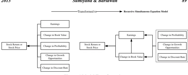
Recursive Simultaneous Model

The model in this study is explained as follows. Classical concept depicts that stock return is associated with earnings yield and book value (Feltham & Ohlson, 1995), while from adaptation theory we can derive invested capital and investment scalability to explain stock return. All those relationship can be drawn schematically as in the Figure 1. Such condition is applicable to recursive simultane-ous model (Gudjarati, 2003). The model will control the bias and inconsistency problem.

Research Model and Hypothesis Develop-ment

(6)

Earnings Yield Earnings yields (Xt) show the value generated from beginning year in-vested assets or equities. Earnings yield is deflated by the opening value of current equity capital which generates current earnings. The increase in earnings yields will increase stock return and vice versa. The increase of stock price is caused by investors’ expectation to obtain future dividend. It be concluded that earnings yield associates with stock price positively (Rao & Litzenberger, 1971; Litzenberger & Rao, 1972; Bao & Bao, 1989; Burgstahler & Dichev, 1997; Collins, et al., 1999; Collins, et al., 1987; Cohen & Lys, 2006; Liu & Thomas, 2000; Liu, et al., 2001; Weiss, Naik and Tsai, 2008; Chen & Zhang, 2007; Ohlson, 1995; Feltham & Ohlson, 1995; Feltham & Ohlson, 1996; Bradshaw, et al., 2006; Abarbanell & Bushee, 1997; Lev & Thiagarajan, 1993; Penman, 1998; Francis & Schipper, 1999; Danielson & Dowdell, 2001; Aboody, et al., 2001; Easton & Harris, 1991; and Warfield & Wild, 1992). Therefore, the alternative hypothesis is stated as follows.

HA1: Earnings yield associates positively with stock return.

Change in Equity Capital The change in equity capital (ΔBt) is the first center of firm value measurement. It is measured by the change in current equity value divided by be-ginning value of current equity. The change in equity value increases because of the increase in earnings, then reflected in the following

book value and stock return. In other words, the change of stock return is in accordance with the change of earnings after denominated by opening value of current capital. It means that change in equity capital associates posi-tively with stock return (Rao & Litzenberger, 1971; Litzenberger & Rao, 1972; Bao & Bao, 1989; Burgstahler & Dichev, 1997; Collins, et al., 1999; Collins, et al., 1987; Cohen & Lys, 2006; Liu & Thomas, 2000; Liu, et al., 2001; Weiss, et al., 2008; Chen & Zhang, 2007; Ohlson, 1995; Feltham & Ohlson, 1995; Feltham & Ohlson, 1996; Bradshaw, et al., 2006; Abarbanell & Bushee, 1997; Lev & Thiagarajan, 1993; Penman, 1998; Francis & Schipper, 1999; Danielson & Dowdell, 2001; Aboody, et al., 2001; Easton & Harris, 1991; and Warfield & Wild, 1992). It is summarized as alternative hypothesis as follows.

HA2.A: Change in firms’ book value associates positively with stock return.

HA2.B: Change in firms’ book value associates positively with earnings yields.

Change in Profitability The change in profitability (Δqt) is the third center of firm value measurement. Change in profitability is perceived by investors as expected future divi-dend. Accordingly, an increase in profititablity is expected to rise future dividend. Such reac-tion is reflected in future stock price increase. On the other side, increase in profitability is caused by the increase in earnings yield. Those earnings subsequently increase book value.

Recursive Simultaneous Equation Model

Stock Return or Stock Price

Earnings

Change in Book Value

Change in Profitability

Change in Growth Opportunities

Change in Discount Rate

Stock Return or Stock Price

Earnings

Change in Book Value

Change in Profitability

Change in Growth Opportunities

Change in Discount Rate Transformed to

(7)

Thus, change in profitability increase as stock return, earning yield, and book value do (Rao & Litzenberger, 1971; Litzenberger & Rao, 1972; Bao & Bao, 1989; Burgstahler & Dichev, 1997; Collins, et al., 1999; Collins, et al., 1987; Cohen & Lys, 2006; Liu & Thomas, 2000; Liu, et al., 2001; Weiss, et al., 2008; Chen & Zhang, 2007; Ohlson, 1995; Feltham & Ohlson, 1995; Feltham & Ohlson, 1996; Bradshaw, et al., 2006; Abarbanell & Bushee, 1997; Lev & Thiagarajan, 1993; Penman, 1998; Francis & Schipper, 1999; Danielson & Dowdell, 2001; Aboody, et al., 2001; Easton & Harris, 1991; and Warfield & Wild, 1992). It is summarized as alternative hypothesis as follows.

HA3.A: Change in profitability associates posi-tively with stock return.

HA3.B: Change in profitability associates posi-tively with earnings yield.

HA3.C: Change in profitability associates posi-tively with book value.

Change in Growth Opportunities Firm’s equity value depends on change in growth opportunities (Δgt). Stock return depends on whether a firm grows or not. If a firm grow, it increases its earnings, equity value and then simultaneously stock return. This growth con-cept is supported by growth adjustment proc-ess using book value and intrinsic value. Be-cause of a growing firm is able to generate earnings from its invested assets, it indicates that assets should have grown in different type of investment than in firms’ equity value. Growth opportunities after being adjusted by relative comparison between book value and intrinsic value associates positively with stock return (Rao & Litzenberger, 1971; Litzenberger & Rao, 1972; Bao & Bao, 1989; Weiss, et al., 2008; Ohlson, 1995; Abarbanell & Bushee, 1997; Lev & Thiagarajan, 1993; Danielson & Dowdell, 2001; and Aboody, et al., 2001). The alternative hypothesis is stated as follows.

HA4.A: Change in growth opportunities as-sociates positively with stock return.

HA4.B: Change in growth opportunities as-sociates positively with earnings yield.

HA4.C: Change in growth opportunities as-sociates positively with book value.

Change in Discount Rate Discount rate shows future cash flow valued by cost of capital. The change in discount rate (Δrt) af-fects future cash flow showed in the earnings and book value, then modifies stock return in turn. The higher discount rate, the lower future cash flow and vice versa. It means that change in discount rate associate negatively with stock price variations (Rao & Litzenberger, 1971; Litzenberger & Rao, 1972; Burgstahler & Dichev, 1997; Liu, et al., 2001; Chen & Zhang, 2007; Feltham & Ohlson, 1995; Feltham & Ohlson, 1996; Danielson & Dowdell, 2001; and Easton & Harris, 1991). It is summarized in the following hypothesis statement.

HA5.A: Change in discount rate associates negatively with stock return.

HA5.B: Change in discount rate associates negatively with earnings yield.

HA5.C: Change in discount rate associates negatively with book value.

RESEARCH METHOD

Population and Sample

(8)

the same certain classification, stock market movement as a respond to accounting infor-mation should be equal.

Sampling Methods

This study uses purposive sampling, the sample is obtained under certain criteria. The criteria (Sumiyana, et al., 2010 and Sumiyana, 2011) are as follows. First, firms are in manu-facture and trading sectors, eliminating finan-cial and banking sectors. This study eliminates financial and banking sectors because they are tightly regulated. Second, opening and closing equity book value must be positive (Bit-1>0;

Bit>0). Firms with negative equity book value tend to go bankrupt. Third, firm stocks are traded actively. Sleeping stocks would disturb conclusion validity.

Variables Measurement and Examination

Variables definition and measurement conducted as follows. Rit is annual stock return for firm i during period t, measured since the first day of opening year period t-1 until one day after financial statement publication or, if any, earnings announcement period t; xit is earnings firm i during period t, calculated by earnings acquired by common stock holders during period t (Xit) divided by equity market value during opening of current period (Vit-1);

1 profitability firm i during period t, deflated by equity book value during opening of current period and profitability calculated using for-mula:

is equity capital or proportional change in equity book value for firm i during period t, adjusted by one minus ratio book value and market value during current period. This ad-justment is needed to balance accounting book value and market value;

1

is change in growth opportunities firm i during period t;

The original model uses model of Chen and Zhang (2007), Sumiyana et al. (2010), and Sumiyana (2011) that is a single equation model. It uses linear regression examination based on model (1). The second examination is recursive on simultaneous equation model (1), (2) and (3). This second examination composes three recursive equations that should be conducted simultaneously as fol-lows.

Constrained with :

Cov. {(eit(1)); (eit(2))} Cov {(eit(1)); (eit(3))} Cov {(eit(2)); (eit(3))} 0

We reexamine the recursive simultaneous equation model with inducing investment scalability (Sumiyana, et al., 2010). This reex-amination splits profitability into short-run and long-run invested asset scalabilities.

1 short-run profitability firm i during period t, deflated by equity book value during opening of current period and profitability. While,

(9)



Constrained with :

Cov. {(eit(4)); (eit(5))} Cov {(eit(4)); (eit(6))} Cov {(eit(5)); (eit(6))} 0

Simultaneous model requires that each re-sidual derived from each linear model should not have the same covariance values with each other. As Gujarati (2003) states that recursive simultaneous model must control its residual errors and its residual covariance between one regression and others to prevent bias. Fur-thermore, linearity examination is conducted for each model and simultaneous equations. The reason is that all models are linear regres-sion and require freedom of normality, hetero-scedasticity, and multicollinearity.

Sensitivity Examination

Sensitivity examination for the recursive simultaneous equation is performed by sample arrangement into various partitions. Partition-ing criteria are ratio between equity book value and stock market value. This examina-tion is aimed to show model consistency within various market levels. Consistency is also expected to be shown at various market changes. Our return model examines consis-tency against systematic risks, and not yet against idiosyncratic risks. The examination is carried out by splitting sample into quintiles according to ratio of book value and market value.

ANALYSIS, DISCUSSION AND FINDINGS

This section describes data analysis, dis-cussion and research findings. It starts with descriptive statistics, analysis, discussion and ends with research findings. Descriptive sta-tistics initiate this analysis.

Descriptive Statistics

Final sample has fulfilled all required cri-teria. This study acquires sample data as much as 6,132 (25.45%) from all population of 24,095 (100.00%). The population comes from all stock market in Asia, Australia and United States of America. The sample data period is 2009. A number of data must be excluded. The number and reason are as follows. First, 8,939 (37.10%) are due to stock price or stock return data incompleteness. Second, 661 (2.74%) are caused by earnings data unavailability. Third, 8,038 (33.36%) are due to expected earnings and growth are not presented. Fourth, 167 (0.69%) are caused by negative earnings. Fifth, 120 (0.50%) are due to extreme data exclusion. Last, 38 (0.16%) are caused by ab-normal return that cannot be calculated using model of Fama and French (1992, 1993, and 1995). This study cannot obtain firms with negative earnings and book value, because their stock price data is incomplete. Therefore, the criteria which exclude firms having nega-tive earnings and book value are automatically accomplished. The acquired data and the ex-clusion are presented in Table 1 as follows.

(10)

Table 1 Sample Data

Number % Number %

1 Population targets 24,095

100.00%

2 Stock price data incomplete 8,939

37.10% 15,156

62.90%

3 Earnings data unavailable 661

2.74% 14,495

60.16%

4 Expected data unavailable 8,038

33.36% 6,457 26.80%

5 Lossing company exclusion 167

0.69% 6,290 26.11%

6 Extreme value exclusion 120 0.50% 6,170 25.61% 7 Inability to calculate abnormal return 38 0.16% 6,132 25.45%

Total 17,963 74.55%

No Note Decrease Sample

Note: Number of valid observation for each country is Indonesia: 59; Malaysia: 326; Australia: 318; China: 976; Hongkong: 67; India: 171; Japan: 1.025; South Korea: 782; New Zealand: 50; Filipina: 38; Singapore: 193; Taiwan: 355; Thailand: 191; and US: 1.578. Mortal country during analysis is Sri Lanka: 3, and mortal countries before initial analysis are Pakistan, Bangladesh and Vietnam.

Table 2 Descriptive Statistics

No. Variable Min. Max. Mean Median Std.

Deviation Perc. - 25 Perc. - 75

1 Ri1 -0.9954 9.8966 0.8463 0.5880 0.9999 0.1667 1.2500

2 Ri2 -0.9964 8.0000 0.4600 0.2419 0.7506 -0.0151 0.7500

3 R_i3 -0.9966 9.0000 0.1627 0.0327 0.5932 -0.1981 0.3689 4 R_i4 -0.9939 6.6310 0.0528 -0.0356 0.5175 -0.2450 0.2186 5 Xit 0.0000 46.2025 0.2092 0.0968 0.9104 0.0532 0.1959

6 -55.1125 58.8148 0.0571 0.0071 1.7100 -0.0313 0.0772 7 -54.3503 33.3750 -0.0873 0.0011 1.7231 -0.0608 0.0553 8 -10.6073 54.4328 0.1977 0.0683 1.2737 0.0056 0.1976 9 -29.9957 28.9790 -0.1362 -0.0737 1.3559 -0.4694 0.0301

10 -506.3845 202.6165 0.0336 0.0907 11.8351 -0.1125 0.4198 11 -250.0161 289.1262 0.2959 0.0609 6.3004 -0.0368 0.2572 12 -54.3503 33.3750 -0.0873 0.0011 1.7231 -0.0608 0.0553

13 PBit 0.0026 70.4000 1.0362 0.6831 2.4254 0.3594 1.2095

14 Vit 0.0100 6,843.3600 39.3251 3.6300 248.8796 1.1600 16.3400

15 Bit 0.0200 4,601.1500 29.8525 2.7450 189.1163 0.5400 10.6200

qit bit git rit srit lrit p_it

Notes: Number of observation (N): 6.132. Rit: stock return for firm i during period 1 (1 year), 2 (1 year 3 months), 3 (1

year 6 months), and 4 (1 year 9 months); xit: earnings for firm i during period t; Δbit: change of book value for firm i

during period t; Δqit: change of profitability for firm i during period t; Δsrit: change of short-run assets scalability for firm i

during period t; Δlrit: change of long-run assets scalability for firm i during period t; Δgit: change of growth opportunities

for firm i during period t; Δrit: change of discount rate during period t;PBit: ratio between stock market value and book

(11)

Since earnings data used in this study are earnings after tax (Xit), it requires firms with profit. Therefore, the minimum value is 0.0000. Mean value is 0.2092, median value is 0.0968, and standard deviation is 0.9104. The median value is in the left side of mean. It shows that there are some firms having enor-mous earnings. However, this condition is not a problem since its standard deviation is less than one. The return data indicates similar tendency. Therefore, the correlation between both variables is possible. The other variables, change of earnings power (Δqit) and change of growth opportunities (Δgit) also show similar tendency as earnings. Meanwhile, change of discount rate shows inversed tendency. Such phenomena are expected.

Recursive Simultaneous Equation Analysis

Recursive simultaneous equation con-structs three main factors –earnings power, growth opportunities and discount rate– which associate consecutively with earnings, book value, and stock return. Then, four main fac-tors; –book value, earnings power, growth opportunities and discount rate– which associ-ate passing through earnings and stock return. Finally, five main factors –earnings yield, book value, earnings power, growth opportu-nities and discount rate– which associate with stock return. They are earnings yield (xit), change in firm book value (Δbit), change in earnings power (Δqit), change in growth op-portunities (Δgit), and change in discount rate (Δrit). The result analysis is presented in Table 3 as follows.

The result shows that earnings (xit), firm book value (Δbit), and growth opportunities (Δgit) are consistently above 1% confirmed that they associate with stock return for vari-ous return specifications (Ri1 until Ri4). They are with t-value (sig.) consecutively 6.785 (1%), 4.770 (1%) and 7.055 (1%) in the Rt1 type and others type of Rt. It means that HA.1, HA.2A, and HA.4A are supported. This study is failed to confirm the association between

earnings power (Δqit) with stock return, unlike Chen and Zhang (2007) who confirm it con-sistently. Meanwhile, change in discount rate (Δrit) is not confirmed. It could be concluded that HA.3A and HA.5A is not supported. Degree of association shows F-value of 35.5187 and significant at level 1%. This basic model has return type R2 of 2.82% for Ri1, and lower for the others. Its adj-R2 value is 2.74%. Mean-while, the first recursive equation has earnings type R2 of 58.2% for xit, and its adj-R2 value is also 58.2%. The second recursive equation has

R2 of 14.3% for change in book value (Δbit) and its adj-R2 value is also 14.3%.

The basic model or the first examination is still able to conclude the association between accounting information and stock return; it is not flexible enough or rigid because the two variables above were not confirmed. There-fore, this result gives sufficient reason for further stage of decomposed examination us-ing recursive equation. Table 1 decomposes earning power (Δqit) in this relationship with stock return. This study successfully proves that power and growth opportunities associate against earnings yields with t-value (sig.) as 48.470 (1%) and 26.266 (1%). It implies that earnings power and growth opportunities then associates with stock return. It means that HA.3B and HA.4B are supported. Even though, this study is still weak because it could not evidence the association between earning power and stocks’ book value. In other words, HA.3C is not supported. Furthermore, HA.5B and HA.5C are also not supported.

(12)

2

013

Sumiyana & B

a

rid

w

a

n

95

Pred. Sign ? + + + +

-Ri1 = 0.810 + 0.145 Xit + 0.045 + 0.000 + 0.077 + 0.037 + eit ……(1) R

2

: 0.028F-Value: 35.519 ***

t-value 61.353 *** 6.785 *** 4.770 *** 0.023 7.055 *** 3.958 Adj-R2: 0.027

Ri2 = 0.445 + 0.052 Xit + 0.028 + 0.007 + 0.044 + 0.016 + eit ……(1) R

2

: 0.011F-Value: 13.513 ***

t-value 44.494 *** 3.194 *** 3.882 *** 1.040 5.299 *** 2.239 Adj-R2: 0.010

Ri3 = 0.155 + 0.020 Xit + 0.019 + 0.008 + 0.025 + 0.000 + eit ……(1) R

2

: 0.005F-Value: 6.041 ***

t-value 19.540 *** 1.576 3.381 *** 1.558 3.762 *** -0.007 Adj-R2: 0.004

Ri4 = 0.042 + 0.040 Xit + 0.026 + 0.002 + 0.025 + 0.002 + eit ……(1) R

2

: 0.009F-Value: 10.915 ***

t-value 6.080 *** 3.552 *** 5.201 *** 0.412 4.342 *** 0.343 Adj-R2: 0.008

Xit = 0.149 + -0.241 + 0.221 + 0.162 + 0.039 + eit ……(2) R

2

: 0.582F-Value:2,134.869 ***

t-value 19.453 *** -51.103 48.470 *** 26.266 *** 6.955 Adj-R2: 0.582

= 0.008 + -0.250 + -0.383 + 0.041 + eit ……(3) R

2

: 0.143F-Value: 341.088 ***

t-value 0.400 -20.982 -23.959 2.713 Adj-R2: 0.143

Constrained with (x 1016):

Cov. {(eit(1)); (eit(2))} = 4.797 0 …….{a} {a}  {b}  {c}  0 Cov. {(eit(1)); (eit(3))} = -3.369 0 …….{b}

Cov. {(eit(2)); (eit(3))} = -1.658 0 …….{c}

Cov. {(eit(1)); (eit(2))} = -0.054 0 …….{a} {a}  {b}  {c}  0 Cov. {(eit(1)); (eit(3))} = -1.249 0 …….{b}

b_it b_it bit b_it bit

git git git git git git

rit rit rit rit rit rit

bit

q_it

qit

(13)

J

o

urna

l of

Indo

nesi

a

n

Eco

n

omy and Business

J

a

nua

ry

Pred. Sign ? + + + + +

-Ri1 = 0.808 + 0.145 Xit + 0.046 + 0.003 + 0.004 + 0.083 + 0.037 + eit…… (1) R

2

: 0.030F-Value: 31.360 ***

t-value 61.470 *** 7.955 *** 4.918 *** 2.666 *** 1.764 * 7.524 *** 4.012 Adj-R2:0.029

Ri2 = 0.443 + 0.060 Xit + 0.029 + 0.001 + -0.001 + 0.046 + 0.016 + eit…… (1) R

2

: 0.011F-Value: 11.617 ***

t-value 44.504 *** 4.360 *** 4.028 *** 1.745 * -0.415 5.494 *** 2.207 Adj-R2:0.010

Ri3 = 0.153 + 0.030 Xit + 0.020 + 0.001 + -0.001 + 0.025 + 0.000 + eit…… (1) R

2

: 0.005F-Value: 5.032 ***

t-value 19.441 *** 2.787 *** 3.541 *** 1.137 -1.070 3.752 *** -0.079 Adj-R2:0.004

Ri4 = 0.042 + 0.042 Xit + 0.026 + 0.001 + -0.002 + 0.027 + 0.002 + eit…… (1) R

2

: 0.009F-Value: 9.786 ***

t-value 6.058 *** 4.394 *** 5.235 *** 1.316 -1.608 4.680 *** 0.318 Adj-R2:0.009

Xit = 0.160 + -0.300 + 0.001 + -0.001 + 0.142 + 0.039 + eit…… (2) R

2

: 0.422F-Value:895.802 ***

t-value 17.823 *** -55.901 1.651 * -0.560 18.796 *** 6.004 Adj-R2:0.422

= -0.001 + -0.006 + -0.011 + -0.391 + 0.042 + eit…… (3) R

2

: 0.085F-Value:141.441 ***

t-value -0.041 -3.125 -3.191 -22.602 2.694 Adj-R2:0.084

Cov. {(eit(4)); (eit(5))} = 5.592 0 …….{d} {d}  {e}  {f}  0

Cov. {(eit(4)); (eit(6))} = -3.961 0 …….{e}

Cov. {(e_it(5)); (e_it(6))} = -6.953 0 …….{f}

Cov. {(eit(4)); (eit(5))} = 0.519 0 …….{d} {d}  {e}  {f}  0

Cov. {(eit(4)); (eit(6))} = -0.586 0 …….{e}

Cov. {(eit(4)); (eit(5))} = 0.525 0 …….{d} {d}  {e}  {f}  0

Cov. {(e_it(4)); (e_it(6))} = -1.178 0 …….{e}

Cov. {(eit(4)); (eit(5))} = 0.278 0 …….{d} {d}  {e}  {f}  0

Cov. {(eit(4)); (eit(6))} = -1.511 0 …….{e} bit bit bit b_it

bit srit

srit

srit lrit lrit lrit lrit lrit lrit

rit rit rit rit rit r_it

bit

(14)

Nevertheless, this examination is not able to support HA.3C, HA.4C, and HA.5C. The second examination or the factoring in the investment scalability model has return type R2 of 3.0% for Ri1, and lower for the others. Its adj-R2 value is 2.9%. Meanwhile, the first recursive equation has earnings type R2 of 42.2% for xit, and its adj-R2 value is also 42.2%. The second recursive equation has R2 of 8.5% for change in book value (Δbit) and its adj-R2 value is also 8.4%.

Sensitivity Examination Results

This study analysis both prior two examinations based on the quartile of PB ratio. Table 5 –panel A– indicates that hypothesis HA1, HA2A, HA3A, and HA5A associated positively with return are supported. This is shown in low PB level for all return types with significance level of 1%, except for Ri2 return type whose significance level of 5%. In the Panel B, C and D, it is also shown in low-medium, medium-high and high PB levels for

Ri1 and Ri4 return types with significance level of, consecutively, 5% and 10%. Meanwhile, HA3A, and HA5A are not supported consistently as the first examination previously. In the low PB level – Panel A, growth opportunities associates positively with earnings yield and earnings power associates positively with book value with t-value (sig.) consecutively as 6.128 (1%) and 3.520 (1%). It means that HA3C and HA4B are supported.

(15)

J

o

urna

l of

Indo

nesi

a

n

Eco

n

J

a

nua

ry

Pred. Sign ? + + + +

-Ri1 = 0.936 + 3.335 Xit + 0.043 + 0.000 + -0.730 + -0.874 + eit …… (1) R

2

: 0.184F-Value: 68.881 ***

t-value 30.616 *** 15.868 *** 2.856 *** -0.001 -11.286 -6.505 *** Adj-R2: 0.182

Ri2 = 0.791 + 0.589 Xit + 0.033 + -0.013 + -0.049 + -0.521 + eit …… (1) R

2

: 0.030F-Value: 9.315 ***

t-value 28.759 *** 3.115 *** 2.437 ** -0.901 -0.851 -4.305 *** Adj-R2: 0.026

Ri3 = 0.464 + 0.341 Xit + 0.021 + -0.002 + -0.002 + -0.466 + eit …… (1) R

2

: 0.029F-Value: 9.014 ***

t-value 20.664 *** 2.210 ** 1.895 * -0.168 -0.043 -4.722 *** Adj-R2: 0.026

Ri4 = 0.207 + 0.488 Xit + 0.021 + 0.005 + -0.069 + -0.268 + eit …… (1) R

2

: 0.026F-Value: 8.263 ***

t-value 10.698 *** 3.677 *** 2.205 ** 0.482 -1.701 -3.160 *** Adj-R2: 0.023

Xit = 0.079 + -0.002 + -0.002 + 0.284 + 0.057 + eit …… (2) R

2

: 0.890F-Value:3,098.040 ***

t-value 25.404 *** -1.036 -1.221 94.991 *** 3.520 Adj-R2: 0.890

= 0.096 + 0.168 + -0.438 + -0.098 + eit …… (3) R

2

: 0.087F-Value: 48.679 ***

t-value 2.212 ** 6.128 *** -10.917 -0.432 Adj-R2: 0.085

Cov. {(eit(1)); (eit(2))} = -9.398 0 …….{a} {a}  {b}  {c}  0

Cov. {(eit(1)); (eit(3))} = 8.408 0 …….{b}

Cov. {(eit(2)); (eit(3))} = -3.373 0 …….{c}

Cov. {(eit(1)); (eit(2))} = -2.183 0 …….{a} {a}  {b}  {c}  0

Cov. {(eit(1)); (eit(3))} = 2.738 0 …….{b}

Cov. {(eit(1)); (eit(2))} = -1.048 0 …….{a} {a}  {b}  {c}  0

Cov. {(eit(1)); (eit(3))} = 0.136 0 …….{b}

Cov. {(eit(1)); (eit(2))} = -1.283 0 …….{a} {a}  {b}  {c}  0

Cov. {(eit(1)); (eit(3))} = 0.676 0 …….{b} bit bit bit b_it b_it

git git g_it git git git

bit

qit

q_it

Additional notes: Number of observation (N): 1,531.

Panel A: Low P/B

(16)

2

013

Sumiyana & B

a

rid

w

a

n

99

Pred. Sign ? + + + +

-Ri1 = 0.837 + 0.145 Xit + 0.051 + 0.010 + 0.727 + -0.026 + eit …… (1) R

2_:

0.063F-Value: 20.696 ***

t-value 26.644 *** 2.052 ** 1.067 0.341 9.355 *** -0.548 Adj-R2:0.060

Ri2 = 0.401 + 0.128 Xit + 0.074 + 0.010 + 0.566 + -0.032 + eit …… (1) R

2

: 0.080F-Value: 26.537 ***

t-value 18.563 *** 2.631 *** 2.244 ** 0.511 10.583 *** -0.999 Adj-R2:0.077

Ri3 = 0.158 + 0.099 Xit + 0.069 + 0.012 + 0.301 + -0.076 + eit …… (1) R

2

: 0.049F-Value: 15.617 ***

t-value 9.172 *** 2.549 *** 2.645 *** 0.769 7.054 *** -2.960 *** Adj-R2:0.046

Ri4 = 0.063 + 0.127 Xit + 0.080 + 0.002 + 0.266 + -0.053 + eit …… (1) R

2

: 0.048F-Value: 15.541 ***

t-value 3.989 *** 3.595 *** 3.332 *** 0.119 6.835 *** -2.279 ** Adj-R2:0.045

Xit = 0.161 + -0.585 + 0.220 + 0.087 + 0.035 + eit …… (2) R

2

: 0.892F-Value: 3,150.104 ***

t-value 15.213 *** -67.101 25.602 *** 3.091 *** 2.099 Adj-R2:0.892

= -0.015 + -0.629 + 0.371 + -0.040 + eit …… (3) R

2

: 0.421F-Value: 371.386 ***

t-value -0.484 -32.508 4.544 *** -0.813 Adj-R2:0.420

Cov. {(e_it(1)); (e_it(2))} = -1.649 0 …….{a} {a}  {b}  {c}  0

Cov. {(e_it(1)); (e_it(3))} = -2.332 0 …….{b}

Cov. {(e_it(2)); (e_it(3))} = 9.352 0 …….{c}

Cov. {(eit(1)); (eit(2))} = -3.531 0 …….{a} {a}  {b}  {c}  0

Cov. {(e_it(1)); (e_it(3))} = -2.888 0 …….{b}

Cov. {(e_it(1)); (e_it(2))} = -1.737 0 …….{a} {a}  {b}  {c}  0

Cov. {(e_it(1)); (e_it(3))} = -0.916 0 …….{b}

Cov. {(e_it(1)); (e_it(2))} = -3.135 0 …….{a} {a}  {b}  {c}  0

Cov. {(eit(1)); (eit(3))} = -1.523 0 …….{b} bit bit bit bit b_it

git git git git git g_it

bit

qit

q_it

qit

qit Panel B: Low-Medium P/B

(17)

J

o

urna

l of

Indo

nesi

a

n

Eco

n

J

a

nua

ry

0

Pred. Sign ? + + + +

-R_i1 = 0.428 + 0.940 X_it+ -0.023 + 0.006 + 0.558 + 0.051 + e_it ……(1) R2_:

0.240F-Value:96.480 ***

t-value 18.864 *** 15.357 *** -1.207 0.292 10.975 *** 3.004 Adj-R2:0.237

R_i2 = 0.158 + 0.498 X_it+ -0.016 + 0.019 + 0.274 + 0.000 + e_it ……(1) R2: 0.147F-Value:52.621 ***

t-value 9.835 *** 11.467 *** -1.166 1.406 7.587 *** -0.027 Adj-R2:0.144

R_i3 = -0.060 + 0.297 X_it+ 0.010 + 0.013 + 0.125 + -0.031 + e_it ……(1) R2_:

0.093F-Value:31.515 ***

t-value -5.109 *** 9.336 *** 0.981 1.283 4.728 *** -3.488 *** Adj-R2:0.091

R_i4 = -0.096 + 0.261 X_it+ 0.028 + 0.010 + 0.123 + -0.023 + e_it ……(1) R2: 0.074F-Value:24.272 ***

t-value -8.069 *** 8.116 *** 2.781 *** 1.014 4.606 *** -2.589 *** Adj-R2:0.071

Xit = 0.163 + -0.066 + 0.083 + 0.161 + 0.016 + eit ……(2) R

2

: 0.141F-Value:62.779 ***

t-value 19.159 *** -8.568 10.653 *** 7.708 *** 2.209 Adj-R2:0.139

= -0.011 + -0.067 + -0.013 + 0.007 + e_it ……(3) R2_:

0.004F-Value: 2.277 *

t-value -0.407 -2.588 -0.183 0.283 Adj-R2:0.002

Cov. {(eit(1)); (eit(2))} = 2.836 0 …….{a} {a}  {b}  {c}  0

Cov. {(eit(1)); (eit(3))} = -0.163 0 …….{b}

Cov. {(eit(2)); (eit(3))} = 4.192 0 …….{c}

Cov. {(eit(1)); (eit(2))} = -0.404 0 …….{a} {a}  {b}  {c}  0

Cov. {(eit(1)); (eit(3))} = -2.425 0 …….{b}

Cov. {(eit(1)); (eit(2))} = -0.223 0 …….{a} {a}  {b}  {c}  0

Cov. {(eit(1)); (eit(3))} = -1.513 0 …….{b}

Cov. {(eit(1)); (eit(2))} = 0.191 0 …….{a} {a}  {b}  {c}  0

Cov. {(eit(1)); (eit(3))} = -0.713 0 …….{b} bit bit bit bit bit

bit

qit

q_it

qit

(18)

2

013

Sumiyana & B

a

rid

w

a

n

10

1

Pred. Sign ? + + + +

-Ri1 = 0.470 + 0.109 Xit + 0.013 + -0.005 + 0.043 + 0.023 + eit ……(1) R

2

: 0.064F-Value: 20.902 ***

t-value 24.346 *** 4.382 *** 1.253 -0.507 4.054 *** 2.951 Adj-R2: 0.061

Ri2 = 0.171 + 0.035 Xit + 0.004 + 0.006 + 0.029 + 0.009 + eit ……(1) R

2

: 0.033F-Value: 10.267 ***

t-value 12.590 *** 1.998 ** 0.560 0.793 3.845 *** 1.714 Adj-R2: 0.029

Ri3 = -0.106 + 0.010 Xit + -0.005 + 0.000 + 0.012 + -0.002 + eit ……(1) R

2

: 0.015F-Value: 4.634 ***

t-value -11.110 *** 0.835 -1.012 0.080 2.385 ** -0.415 Adj-R2: 0.012

Ri4 = -0.153 + 0.025 Xit + 0.005 + -0.008 + 0.015 + 0.001 + eit ……(1) R

2

: 0.021F-Value: 6.476 ***

t-value -16.906 *** 2.162 ** 1.005 -1.727 3.033 *** 0.351 Adj-R2: 0.018

Xit = 0.171 + 0.251 + -0.223 + 0.196 + 0.046 + eit ……(2) R

2

: 0.670F-Value: 775.065 ***

t-value 8.829 *** 29.496 *** -23.818 20.325 *** 5.765 Adj-R2: 0.669

= -0.132 + -0.319 + -0.450 + 0.044 + eit ……(3) R

2

: 0.256F-Value: 175.574 ***

t-value -2.505 -14.681 -19.028 2.053 Adj-R2: 0.255

Cov. {(eit(1)); (eit(2))} = -3.625 0 …….{a} {a}  {b}  {c}  0 Cov. {(eit(1)); (eit(3))} = 7.495 0 …….{b}

Cov. {(eit(2)); (eit(3))} = -10.758 0 …….{c}

Cov. {(eit(1)); (eit(2))} = 0.264 0 …….{a} {a}  {b}  {c}  0 Cov. {(eit(1)); (eit(3))} = 0.532 0 …….{b}

Cov. {(eit(1)); (eit(2))} = 0.510 0 …….{a} {a}  {b}  {c}  0 Cov. {(eit(1)); (eit(3))} = 1.809 0 …….{b}

bit bit bit bit bit

bit

qit

q_it Panel D: High P/B

(19)

The second sensitivity examination was conducted by using factoring in the investment scalability in to P/B partition. Consistent with previous examinations, Table 6 – Panel A shows results that earnings yields and book value associate positively with variations of stock price with t-value (sig.) as 15.868 (1%) and 2.856 (1%). In this section, we find a new supported hypothesis that discount rate associ-ate negatively with movements of stock price with t-value (sig.) as -6.505 (1%). It means that HA1A, HA2A, and HA5A are supported. Ex-amination using sample partition based on low-medium PB and medium-high PB levels shows that hypothesis HA5A which states that discount rate associates negatively with stock price is supported, either in panel B and C.

The first recursive simultaneous model in Table 5 – Panel A shows that earnings yield relates only to growth opportunities with R2 of 89.0% and higher than the others. Its adj-R2

value is also 89.0%. The book value is shown to associate with earnings power with R2 of 8.7%. Its adj-R2 value is also 8.5%. However, this association has higher degree of associa-tion in low-medium P/B and high P/B with R2

and adj-R2 value, consecutively, 42.1% and 42.0% for low-medium P/B, and 25.6% and 25.5% for high P/B.

Table 6 – Panel A also shows results that growth opportunities associates positively with earnings yield with t-value (sig.) as 94.991 (1%). We find that HA4B is supported. In addi-tion, earnings power associates positively with

earnings yield with t-value (sig.) as 6.218 (1%). It could be concluded that HA3C is sup-ported. In the Panel B, we find that growth opportunities associate positively with book value with t-value (sig.) as 5.858 (1%). We find that HA4C is supported. Furthermore, long-run investment scalability associates with book value with t-value (sig.) as 1.861 (10%) that supports to the hypothesis HA3C. Table 6 – Panel C and D did not document additional results as Table 6 – Panel A and B.

The second sensitivity examination as pre-sented in Table 6 – Panel A shows that earn-ings yield relates to long run scalability and growth opportunities with R2 of 89.1% and higher than the others. Its adj-R2 value is also 89.0%. The book value is shown to relate with other factors insignificantly, except for low-medium P/B (Panel B). It shows significant association with long run scalability and growth opportunities with R2 and adj-R2 value, consecutively, 2.5% and 2.2%.

(20)

2

013

Sumiyana & B

a

rid

w

a

n

10

3

bit bit bit bit

bit srit

srit

srit lrit lrit lrit lr_it lrit lrit

Pred. Sign ? + + + + +

-Ri1 = 0.934 + 3.354 Xit + 0.043 + 0.000 + -0.015 + -0.713 + -0.870 + eit …… (1) R

2

: 0.185F-Value: 57.739 ***

t-value 30.574 *** 15.934 *** 2.905 *** -0.135 -1.350 -10.971 -6.506 *** Adj-R2:0.182

Ri2 = 0.790 + 0.610 Xit + 0.031 + -0.001 + -0.013 + -0.045 + -0.506 + eit …… (1) R

2

: 0.030F-Value: 7.988 ***

t-value 28.732 *** 3.221 *** 2.337 ** -0.668 -1.309 -0.766 -4.204 *** Adj-R2:0.027

Ri3 = 0.464 + 0.355 Xit + 0.021 + 0.001 + -0.009 + 0.008 + -0.463 + eit …… (1) R

2

: 0.030F-Value: 7.767 ***

t-value 20.640 *** 2.292 ** 1.906 * 0.436 -1.164 0.168 -4.707 *** Adj-R2:0.026

Ri4 = 0.206 + 0.486 Xit + 0.022 + 0.000 + 0.000 + -0.066 + -0.273 + eit …… (1) R

2

: 0.026F-Value: 6.861 ***

t-value 10.684 *** 3.655 *** 2.307 ** 0.340 0.019 -1.605 -3.222 *** Adj-R2:0.022

Xit = 0.079 + -0.002 + 0.000 + 0.003 + 0.278 + 0.058 + eit …… (2) R

2

: 0.891F-Value:2,486.568 ***

t-value 25.523 *** -1.265 -0.202 2.608 *** 80.597 *** 3.595 Adj-R2:0.890

= 0.083 + 0.000 + 0.006 + -0.369 + -0.242 + eit …… (3) R

2

: 0.065F-Value: 26.491 ***

t-value 1.885 * -0.163 0.334 -7.735 -1.060 Adj-R2:0.062

Cov. {(eit(4)); (eit(5))} = -8.807 0 …….{d} {d}  {e}  {f}  0

Cov. {(eit(4)); (eit(6))} = 7.856 0 …….{e}

Cov. {(eit(5)); (eit(6))} = -3.116 0 …….{f}

Cov. {(eit(4)); (eit(5))} = -2.227 0 …….{d} {d}  {e}  {f}  0

Cov. {(eit(4)); (eit(6))} = 1.954 0 …….{e}

Cov. {(eit(4)); (eit(5))} = -0.852 0 …….{d} {d}  {e}  {f}  0

Cov. {(eit(4)); (eit(6))} = 0.256 0 …….{e}

Cov. {(eit(4)); (eit(5))} = -1.320 0 …….{d} {d}  {e}  {f}  0

Cov. {(eit(4)); (eit(6))} = 0.114 0 …….{e} b_it

Table 6 Recursive Simultaneous Equation Analysis – Factoring in the Scalability – P/B Partition

Panel A: Low P/B

(21)

J

o

urna

l of

Indo

nesi

a

n

Eco

n

J

a

nua

ry

4

g_it g_it git git git git

lrit lrit lrit lrit lrit lrit srit

srit

sr_it

srit bit

bit bit b_it bit

Pred. Sign ? + + + + +

-Ri1 = 0.830 + 0.163 Xit + 0.058 + 0.008 + 0.007 + 0.717 + -0.027 + eit ……(1) R

2

: 0.065F-Value: 17.629 ***

t-value 26.736 *** 2.730 *** 1.224 1.234 0.900 9.207 *** -0.573 Adj-R2:0.061

Ri2 = 0.398 + 0.137 Xit + 0.075 + 0.009 + -0.003 + 0.556 + -0.033 + eit ……(1) R

2

: 0.082F-Value: 22.812 ***

t-value 18.639 *** 3.336 *** 2.315 ** 1.990 ** -0.479 10.378 *** -1.044 Adj-R2:0.079

Ri3 = 0.155 + 0.115 Xit + 0.073 + 0.001 + 0.000 + 0.298 + -0.078 + eit ……(1) R

2

: 0.048F-Value: 12.928 ***

t-value 9.115 *** 3.502 *** 2.836 *** 0.381 -0.056 6.968 *** -3.033 *** Adj-R2:0.045

Ri4 = 0.064 + 0.125 Xit + 0.078 + 0.001 + -0.004 + 0.265 + -0.054 + eit ……(1) R

2

: 0.049F-Value: 13.166 ***

t-value 4.094 *** 4.194 *** 3.304 *** 0.348 -1.080 6.790 *** -2.300 ** Adj-R2:0.045

Xit = 0.171 + -0.726 + 0.003 + -0.016 + 0.087 + 0.007 + eit ……(2) R

2

: 0.848F-Value:1,703.955 ***

t-value 13.595 *** -91.098 1.151 -4.904 2.593 *** 0.344 Adj-R2:0.847

= -0.063 + -0.011 + 0.020 + 0.621 + 0.068 + eit ……(3) R

2

: 0.025F-Value: 9.770 ***

t-value -1.565 -1.247 1.861 * 5.858 *** 1.066 Adj-R2:0.022

Cov. {(eit(4)); (eit(5))} = -2.847 0 …….{d} {d}  {e}  {f}  0

Cov. {(eit(4)); (eit(6))} = -1.570 0 …….{e}

Cov. {(eit(5)); (eit(6))} = 4.567 0 …….{f}

Cov. {(e_it(4)); (e_it(5))} = -4.184 0 …….{d} {d}  {e}  {f}  0 Cov. {(eit(4)); (eit(6))} = -1.265 0 …….{e}

Cov. {(eit(4)); (eit(5))} = -2.179 0 …….{d} {d}  {e}  {f}  0

Cov. {(eit(4)); (eit(6))} = -0.319 0 …….{e}

Cov. {(eit(4)); (eit(5))} = -3.432 0 …….{d} {d}  {e}  {f}  0

Cov. {(eit(4)); (eit(6))} = -0.899 0 …….{e} b_it

(22)

2

013

Sumiyana & B

a

rid

w

a

n

10

5

Panel C: Medium-High P/B

Pred. Sign ? + + + + +

-Ri1 = 0.426 + 0.940 Xit + -0.022 + -0.004 + 0.007 + 0.550 + 0.051 + eit …… (1) R

2

: 0.245F-Value:82.537 ***

t-value 18.910 *** 15.950 *** -1.149 -1.171 2.928 *** 10.754 *** 3.001 Adj-R2: 0.242

Ri2 = 0.156 + 0.513 Xit + -0.015 + 0.000 + 0.004 + 0.259 + -0.001 + eit ……. (1) R

2

: 0.150F-Value:44.820 ***

t-value 9.741 *** 12.243 *** -1.122 -0.125 2.657 *** 7.132 *** -0.088 Adj-R2: 0.146

Ri3 = -0.061 + 0.309 Xit + 0.010 + 0.001 + 0.000 + 0.119 + -0.031 + eit ……. (1) R

2

: 0.093F-Value:26.002 ***

t-value -5.209 *** 10.032 *** 0.972 0.560 0.077 4.459 *** -3.543 *** Adj-R2: 0.089

Ri4 = -0.097 + 0.270 Xit + 0.027 + 0.001 + -0.001 + 0.119 + -0.023 + eit ……. (1) R

2

: 0.073F-Value:20.169 ***

t-value -8.150 *** 8.711 *** 2.760 *** 0.680 -0.551 4.415 *** -2.632 *** Adj-R2: 0.070

Xit = 0.167 + -0.071 + -0.003 + 0.000 + 0.150 + 0.013 + eit …… (2) R

2

: 0.079F-Value:26.247 ***

t-value 19.016 *** -8.938 -1.679 0.326 6.879 *** 1.828 Adj-R2: 0.076

= -0.015 + 0.003 + -0.003 + 0.001 + 0.008 + eit …… (3) R

2

: 0.001F-Value: 0.291

t-value -0.518 0.490 -0.881 0.011 0.361 Adj-R2: -0.002

Constrained with (x 1016_):

Cov. {(e_it(4)); (e_it(5))} = 2.209 0 …….{d} {d}  {e}  {f}  0

Cov. {(eit(4)); (eit(6))} = -2.937 0 …….{e} Cov. {(eit(5)); (eit(6))} = 5.450 0 …….{f}

Cov. {(eit(4)); (eit(5))} = 0.185 0 …….{d} {d}  {e}  {f}  0 Cov. {(eit(4)); (eit(6))} = -2.627 0 …….{e}

Cov. {(eit(4)); (eit(5))} = 0.148 0 …….{d} {d}  {e}  {f}  0 Cov. {(eit(4)); (eit(6))} = -1.202 0 …….{e}

Cov. {(eit(4)); (eit(5))} = 0.281 0 …….{d} {d}  {e}  {f}  0 Cov. {(e_it(4)); (e_it(6))} = -0.876 0 …….{e}

git lrit

git git git git git

lrit lrit lrit lrit lr_it

b_it b_it bit bit b_it

b_it

srit