FOOD DEMAND IN YOGYAKARTA:
SUSENAS 2011
Agus Widarjono
Department of Economics
Faculty of Economics Universitas Islam Indonesia
Email: [email protected]
Abstract
The impacts of economic and demographic variables on food demand in Yogyakarta are estimated using the Almost Ideal Demand System (AIDS). Data from the national social and economic survey of households (SUSENAS) in 2011 are used to accomplish the goal of this study. Food demand consists of cereals, sh, meats, eggs and milk, vegetables, fruits, oil and fats, prepared foods and drinks, other foods and tobacco products. Results show that except for meat and tobacco products, demand elasticities for the rest of foods are inelastic and cereals is the least responsive to price change. All ten studied foods are normal good, but their income elasticities are very inelastic.
Keyword:Almost Ideal Demand System (AIDS), price and income elasticity, Yogyakarta.
1. INTRODUCTION
Inflation in Special Region of Yogyakarta province and hereafter it is called Yogyakarta for the rest of the paper over 2009-2011 was stable below two digits but relatively high in 2010. Inflation rates during those three years were 2,98 %, 7.38 % and 3.88 % respectively. However, interestingly food groups significantly contributed inflation during those years. Inflation rate of food stuffs were 3.91 %, 18.06 % and 1.82 % while inflation rate of prepared food, beverage and tobacco products products were 7.81 %, 6.96 %, and 4.51 % over 2009-2011. When we look at detail in subgroup of food stuffs, contribution of inflation rate of cereals, cassava and their product, preserved fish, vegetables, fruits, species, and fats and oil to inflation rate in 2010 were relatively high by 18.92%, 17.18%, 44.40%, 27.01%, 59.89% and 15.89%. Even though inflation rate went down in 2011, the inflation rate of cereals, cassava, and their product, preserved fish and fats and oils were still high by 11.75%, 8.87% and 7.41%. The contribution of subgroup prepared food, beverage and tobacco products mainly came from tobacco products and alcoholic beverages to inflation in Yogyakarta in 2010 by 8.32 % and increased to 12.23% in 2011 (CBS Yogyakarta, 2011).
An increase in food prices definitely influence society welfare in Yogyakarta because foods are a basic human need. Households certainly reduce food consumption and also substitute from high quality to low quality foods. As results, high food prices affect not only poverty but also malnutrition. Several demand studies have been conducted to examine food demand in Indonesia. Moeis (2003) using LA/AIDS (linear approximation Almost Ideal Demand system) analyze on the impact of the 1997/1998 economic crisis on demand for food. Widodo (2004) using linear expenditure system (LES) estimated Indonesian food demand model using seven rounds of survey of living cost. Fabiosa et al. (2005) with an incomplete demand system (LinQuad) estimated food demand using 1996 SUSENAS data . Unlike other food demand studies using SUSENAS data set and LA/AIDS model, Pangribowo and Tsegai (2011) estimated demand for foods from Indonesia Family Life Survey (IFLS). The purpose of this study is to estimate the demand for foods in Yogyakarta. This study differs the previous studies. First, this study uses the latest SUSENAS in 2011 for specific area at province level instead of whole country. Second, the LA/AIDS using a linear
elasticities (Alston et al. 1994). This study estimate demand for food in Yogyakarta with the non-linear AIDS model. The analysis of food demand in Yogyakarta is expected to be one of the important information to local governments in the Yogyakarta in formulating food policy.
The rest of this paper is organized as follows. Section II discusses food consumption patterns in Central Java. Model of household food demand and data in Yogyakarta are presented in the following section. The next section discusses estimation procedures and results. The final section of this study presents some conclusions.
2. FOOD CONSUMPTION PATTERNS IN YOGYAKARTA
Household expenditure is one of the most important components of aggregate demand determining economic activity in a region. In addition, the social welfare can also be measured from the level of household expenditures. The higher household expenditure is the higher the level of society welfare. Household expenditure can be divided into two major groups, namely food and non-food expenditures. During the year 2011, the per capita household expenditures in Yogyakarta were Rp 625,043 consisting of food and non-food expenditure by Rp 276,325 and Rp 348,721 respectively. Whereas per capita household expenditure in 2010 were Rp 553,967 which expenditures of food and non-food respectively were Rp 244,004 and Rp 309,963. Per capita expenditures increased by 12.83 percent in 2011 driven by spending on food groups by 13.25 % and non-food group by 12.50%. When viewed by area of residence, per capita expenditures of urban households in 2011 were Rp 702,787 or increasing by 7.10 % compared to in 2010 that were only Rp 656,190. By contrast, the per capita expenditures of the rural population in 2011 were only Rp 472,165 but its growth was higher by 27.64% (CBS Yogyakarta, 2011). Per capita expenditure urban households were higher than the expenditure of the rural households during 2010-2011, so that on average the welfare of the urban families were better than the rural families in both years.
Household spending patterns will shift with increasing income. The higher income leads to decreasing the share of expenditure on foods and increasing share of expenditure on non-foods. In 2010, the percentage of food expenditure to the total expenditure was 44.05% and increased to 44, 21% in 2011. On the other hand, non-food expenditure share to total expenditure during 2010-2011was 55.95% and 55.79% respectively. The portion of non-food expenditure to total consumption in urban areas was still higher than the non-food groups in the amount of 58.72 percent and 56.89 percent in 2010 and 2011. However, expenditures on food were still relatively higher in rural areas as compared to non-food expenditures by 52.88% and 47.12% respectively in 2010. However, the opposite condition occurred in 2011 in which the non-food expenditures (52.57%) were higher than the food expenditures (47.43%) (CBS Yogyakarta, 2011).
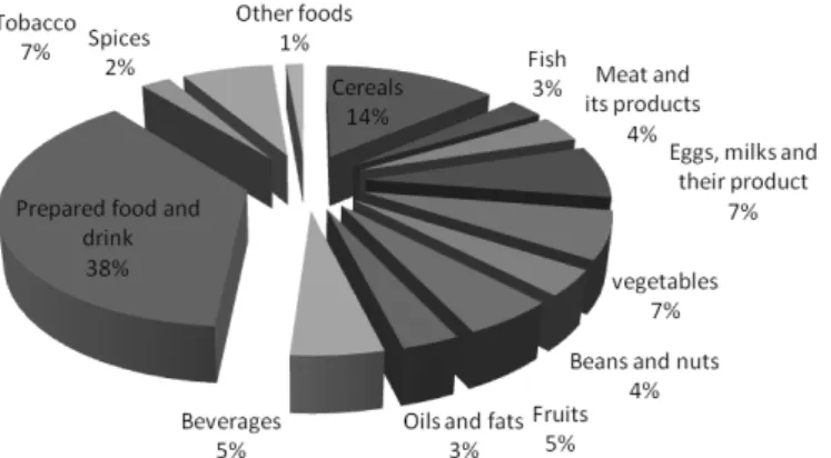
Source: CBS Yogyakarta, 2011
Figure 1 presents the distribution of food expenditures per capita population in 2010. Expenditures on prepared food and drink mostly contributed to total food expenditures by 38%. Large expenditure share for prepared food and drink related to those resident who rent house especially students whom their consumption patterns tend to buy fast foods. Cereals with subgroups such as rice, cassava, maize (14%) also significantly contributed to total food expenditures. Expenditures on dairy product such as eggs, milk and their product and vegetables were 7%. However, spending on high-value foods from meat and its product, fish, oils and fats were relatively low by less than 3%. More interestingly share of tobacco products expenditure to total expenditure were relatively high (7%).
3. MODEL SPECIFICATION AND DATA
3.1. Model Speci cation
This study estimates demand foods in Yogyakarta. The demand for foods encompass cereals, fish, meat, eggs and milk, vegetables, fruits, oil and fats, prepared food and drink, other foods, and tobacco products. To estimate demand for ten food groups in Yogyakarta, we begin with the classical utility maximization framework. Economists use the concept of utility to define the level of satisfaction that comes from a specific allocation of income among different products. The basis of demand analysis is the problem of how to maximize utility subject to a given level of income. This can be expressed as:
(1)
where U is a utility function of the quantities of goods consumed, Y is total income, p and q are prices and quantities, respectively.
The solution to the equation (1) gives the amount demanded of each good as a function of its price, price of other goods and the consumer’s income. The problem exists for the empirical analyst when the number of good involved is too large. Some alternative approaches were proposes to solve. One is the composite commodity theorem that groups commodities based on the behavior of their relative prices. The others are separability and two-stage budgeting that makes assumption about the consumer’s preferences.
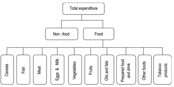
This study uses separability and two-stage budget procedures to analyze the demand for ten foods in Yogyakarta. Following Deaton and Muellbaur (1980), Weak separability is important for the second stage of two budgeting in demand system’s analysis. If food is assumed to be weakly separable from non-food, then the consumer’s utility maximization decision can be decomposes into two stages budget procedures. In the first-stage budgeting, total expenditure is allocated among food and non food items. Food expenditure is then allocated among the studied foods. Figure 1 shows the utility tree of a representative Yogyakarta households in analyzing demand for foods.
Figure 2. Household Utility Tree for foods Consumption in Yogyakarta
The Working (1943)-Leser (1963) food demand is chosen in the first-stage budgeting to estimate demand ealsticity for food and written as:
(2)
where i and j are goods, wi is the share of total expenditure allocated to the i th good, pj is the price of the j th good, is the household expenditures on goods, Mk is the demographic variables consisting of urban, household size, years of schooling of household head, age of household head, gender of household head, and two quarter dummy variables (Quarter 2 and quarter 3).
From equation (2), we can derive uncompensated (Marshallian) price and expenditure elasticities. Uncompensated price ∈ij and expenditure ∈i elasticities are:
(3)
(4)
where is the Kronecker Delta that is zero if ≠ and unity otherwise. Own-price, cross-price and expenditure elasticity are evaluated at sample means. Because the Working-Lesser does not provide a direct estimate of income elasticity, this study uses Engle function as follow:
where is the household expenditures on foods, X is total expenditure on food and non-food, P is price index of foods, and Zk is the demographic variables that are same as previously defined in equation (2). The income elasticity is estimated as (Chern et al, 2003):
(6)
In the second-stage budgeting a almost ideal demand system (AIDS) developed by Deaton and Muellbauer (1980) is used to analyze demand for ten food groups. The AIDS model is
(7)
where i and j are goods, wi is the share of total expenditure allocated to the i th good, Pj is the price of the j th good, X is the household expenditure on goods in the system, a(P) is the price index, γij, i, and (i are parameters to be estimated, and ui is an error term. The price index a (P) is
The demand for food is influenced not only economic variables but also demographic variables. To capture demographic variables in estimating demand for food, we incorporate demographic variables into the intercept in equation (7) as defined i = (i0 + (k = 1) m (ik dk where dk is the demographic variables consisting urban, of household size, educational level of household head (years of schooling), age of household head, gender of household head, and two quarter dummy variables (Quarter 2 and quarter 3).
Because expenditure variables in the AIDS model are endogenous variable, it likely happens that error terms and expenditure variable in equation (7) is correlated and lead to biased parameter estimates. The two-step estimations proposed by Blundell and Robin (1999) is applied to correct for the endogeneity problem in the AIDS model. The first step is to run the following equation:
lnY = H + e (8)
Where Y is total food expenditure of the studied food groups and H a set of explanatory variables encompassing of income, square of income, prices of the studied goods, and demographic variables that are used in equation (7). Total household expenditure is used as a proxy for income (Deaton, 1996; Moeis, 2003). Assuming E (vi|H,e) = 0, residual ê from the first step are incorporated into equation (7) as follow:
ui = (i ˆ + vi (9)
Following Deaton and Muellbauer (1980), the properties of classical demand theory can be imposed on AIDS model. The adding-up restriction is given as:
Homogeneity is imposed as:
(11)
Slutsky symmetry is given as:
γ
ij =
γ
ji, i
≠
j.
(12)
3.2 Data
This study used the national social and economic survey of household in Indonesian (SUSENAS) in 2011 from quarter 1 to quarter 3. The total sample of households in the 2011 SUENAS for Yogyakarta consists of 2,714 households from 1 city and 4 regencies encompassing Yogyakarta City, Sleman, Kulonprogo, Bantul and Gunung Kidul respectively. SUSENAS in 2011 provides food and non-food expenditures. Food expenditures consist of 225 food commodities. For the purpose of this study, we classify to 10 food groups encompassing: (1) cereals (2) fish; (3) meat; (4) eggs and milk; (5) vegetables; (6) fruits; (7) oil and fats; (8) prepared food and drink ;(9) other foods; and (10) tobacco products. Non-food expenditures consist of 6 commodity groups encompassing housing and household facility, goods and services, clothing, footwear, and headgear, durable goods, taxes and insurance, and parties and ceremony.
In the first-stage budgeting, food and non-food demand are estimated using monthly food and non-food expenditures data. The 2011 SUSENAS provides information prices for each food commodities. Weighted average of price within groups using budget share as a weight is used to calculate aggregate price for each food groups (Moschini,1995). Since information prices for non-food expenditures are not available in the 2011 SUSENAS, consumer price indexes in every regency/city are used to calculated non-food price (Jensen and Manrique, 1998).
In the second-stage budgeting, this study estimate demand for ten food groups. Weekly food expenditures data are used in estimating food demand. Estimating demand system requires complete price information. If missing or unreported aggregate price exists in the second-stage budgeting, this price is calculated by regressing observed prices on four regional dummies (Kulonprogo, Bantul, Yogya City and Sleman), seasonal dummies (quarter 2 and quarter 3), and income ( Heien and Wessells,1988). The SUSENAS in 2011 reports household income but missing income data for Yogyakarta are 25.09 % of total sample. Total household expenditure, therefore, is used as a proxy for income (Deaton 1996; Moies, 2003).
4. ESTIMATION AND RESULTS
4.1. Estimation Procedures
As previously discussed, in the first-stage budgeting total expenditure are allocated between food and non-food expenditure. The household survey reported by the SUSENAS reports both non-food and non-non-food expenditure. However, the SUSENAS provides some zero expenditures in given type food expenditures in the second-stage budgeting. Unavailable data from the 2011 SUSENAS for cereals, fish, meats, eggs and milk, vegetables, fruits, oil and fats, prepared foods and drinks, other foods and tobacco products are 11.13%, 57.77%, 56.82%, 20.93%, 15%, 20.93%, 13.85%, 9.73% and 48.31% respectively for Yogyakarta. Prepared food and drink group has no zero expenditures. The non-purchase for given food might be due to no preference, infrequency of purchase, and survey error during survey period.
Zero expenditures imply that the demand system are the limited dependent variables or censored model and leads to biased estimation (Heien &Wessels 1990). Since data in the second-stage budgeting except for prepared food and drink group indicate some zero expenditures, the AIDS model must account for zero expenditures. The
biased estimation for a system of equations with limited dependent variables in the demand system can be solved by using the consistent two- step estimation procedure for cereals, fish, meats, eggs and milk, vegetables, fruits, oil and fats, other foods and tobacco products proposed by Shonkwiler and Yen (1999). Probit model is applied to determine the probability of buying a given type of food group in the first-step estimation. Because it is possible correlation among the different foods, this study employs the multivariate probit regression (Pan, Monhanty, and Welch, 2008). In this case, the multivariate Probit regression is estimated simultaneously for the ten food groups. The explanatory variables are the logarithms of prices of the ten studies food groups, the logarithms of total household expenditure and demographic variables that are same as those used in equation (7). The probit regression is defined as :
prob (yit = 1| Zh ) = 1 - ((Zh(τi) (13) prob (yit = 0| Zh ) = 1 - ((Zh(τi) (14) where Zh is a vector of explanatory variables in probit estimation and τi is the vector of associated parameters for the commodities in probit estimation.
Both the estimated standard normal probability density function (PDF) and the estimated standard normal cumulative distribution function (CDF) from the first-step estimation are augmented in the AIDS model. Finally, the AIDS model in the second-stage budgeting is (Shonkwiler &Yen 1999):
wi = {i + ( j = 1)n γij lnpj + i ln (X / (P) ) + ui }( (.) + τ (.) + i (15) where ( and () are cumulative distribution function (cdf) and probability distribution function (pdf), respectively. Incorporating ( and into the system of equation (15) in the second step estimation causes heteroscedasticity (Shonkwiler&Yen 1999). This heteroskedasticity in the second-step estimation of demand system leads to inefficient but consistent parameter estimates (Shonkwiler and Yen, 1999; Green, 2012).
The Marshallian price and expenditure elasticities of the AIDS model with censoring model in the second-stage budgeting are calculated as follows:
eij = 1/ Wi {γij - i (ih + ( j = 1)n γij lnpj ) } (i - (ij (16)
ei = 1 + 1/ Wi [ i ] (i ei = 1 + 1/Wi [ i ] (i (17)
where eij and ei are Marshallian price and expenditure elasticities, (ij is the Kronecker delta (1 if i = j and 0 otherwise).
The price and expenditure elasticities are computed on the basis of parameter estimated and sample means of independent variables using equation (16) and (17) and the delta method is used to calculate standard errors of both price and expenditure elasticities.
Demand elasticity for price and expenditure elasticities of demand for ten food groups in the second-state budgeting are conditional on total food expenditure in the first-stage budgeting. Unconditional price (σij) and expenditures (ωi ) elasticities are calculated following procedures proposed by Edgerton (1997) and are given as:
(i j = eij + ei [w j + ʲij w j ] (18)
where eij is the conditional Marshallian price elasticity, ei is the conditional expenditure elasticity for j th food groups, ʲij is the Marshallian price elasticity of food in the first-stage budgeting, wj is the expenditure share of j th food groups, and ʲi is the unconditional expenditure elasticity for food in the first-stage budgeting. Finally, following Park et al (1996) the income elasticity for i th food groups is given:
(i = (i ʲy (i = (i ʲy (20)
where (i is the unconditional expenditure elasticity for i th commodity within food groups and (y the income elasticity of food in the first-stage budgeting.
4.2. Results and Discussion
There are only two broad commodity groups for the first stage of the demand system: food and non-food commodity and the second stage consists of ten commodities within the food group: cereals, fish, meats, eggs and milk, vegetables, fruits, oil and fats, prepared food and drink, other foods and tobacco products. The Working-Leser is estimated by the Ordinary Least Squares (OLS). The first stage demand system results an unconditional price and expenditure elasticities of food. The results for the first-stage commodity groups show that own-price, expenditure and income elasticity of food are -0.925; 0.68; and 0.376 respectively. Meanwhile, own-price, expenditure and income elasticity of food are -0,202; 1.356; and 0.793. Demand are less price elastic for both food and food in Yogyakarta. Income elasticities for food and food are all less than one. Therefore, both food and non-food are necessity good but non-food are less elastic than non-non-food1.
Table 1 represent probit estimation for nine food groups except prepared food and drink since the prepared foods and drinks have no zero expenditures. As previously mentioned, there are three explanatory variables namely demographic, price and income variables that affect the probability of buying food in probit model. Among 61 demographic variables, 31 variables are statistically significant at 10% or lower levels but gender and dummy variable for quarter 2 and 3 do not influence strongly demand for the ten foods. 41 of 90 price variables are statistically significant at 10% or lower levels. Of 9 expenditure variables, 7 variables are statistically significant at 10% or lower levels. In general, most of explanatory variables ( 54.97%) in the probit model are statistically significant. Therefore, demographic, price and income variables play a important role in determining whether household buy or not foods in Yogyakarta.
The second step the AIDS model includes PDF and CDF from the first step probit model for food demand and is estimated by Full Information Maximum Likelihood (FIML) estimation with imposition of homogeneity and symmetry. Table 2 reports estimated parameters of the AIDS demand system for food demand in Yogyakarta. 9 of 10 parameter estimates for the standard normal PDF in the AIDS model are statistically significant at the 1% level. These results indicate that the probability of buying a given type of food groups for those households who did not buy foods during survey period exists. These findings provide strong evidence that zero observations must be included in estimating demand for food in Yogyakarta. The Dependent variables in the AIDS demand system are expenditure share and the explanatory variables consists of economic (price and expenditure) and demographic variables. Among 100 price variables, 79 price coefficients (79%) are statistically significant at 10% or lower levels. Of 10 expenditure variables, all expenditure variables are statistically significant at 10% or lower levels. Among 70 demographic variables, 52 (72.29%) variables are statistically significant at 10% or lower levels. Therefore, including demographic variables could explain better demand for food in Yogyakarta
Table 3 reports the full matrix of the conditional Marshallian (uncompensated) price and expenditure elasticities for the 10 food groups. All price and expenditure elasticities are evaluated on the basis of parameter estimated and sample means of independent variables using equation (16) and (17). Standard errors of both price and expenditure elasticities are calculated using the delta method. The diagonal elements in table 4 are own-price elasticities. All own-price elasticities are negative and statistically significant at 1% level. The estimated conditional 1 We don’t report regression results. The complete results are available upon request
Marshallian cross-price elasticities are indicated by the non-diagonal elements in table 4. Among 90 cross-price elasticities, 72 cross-price elasticities are statistically significant at 10% or lower levels. The last row of table 4 presents the estimated conditional expenditure elasticities. All conditional expenditure elasticities are positive and statistically significant at 1% level.
Of interest demand elasticity is unconditional demand elasticity because demand for foods are conditional on demand for all commodities. The unconditional Marshallian price and expenditure elasticities are shown in Table 4. Unconditional demand elasticity is calculated using equation (18) and (19). All own-price elasticities are negative and range from -0.429 for cereals to -1.463 for meat. These results indicate that food demands in Yogyakarta are consistent with economic theory. All own-price elasticities are less than unity, except for meat and tobacco products. demand for cereals is least responsive to price change. On other hand, demand for meat is most responsive food groups to price change. As expected, these results are consistent with the diary habits of consumer in Yogyakarta because cereals with rice as one of subgroups is a basic food and meats are not a main dish. The signs of cross-price elasticities show the studied food products are a mixture of gross substitutes and complements. Fish category, for instance, is a gross substitute for cereals, vegetable, oils and fats, other foods but it is a gross complement for, eggs and milk, fruits, prepared foods and drinks, and tobacco products category. Egg and milk category is a gross substitute for cereals, meat, oils and fats, other foods, and tobacco products, but it is a gross complement for, fish, fruits, vegetables, and prepared foods and drinks. All unconditional expenditure elasticities are positive and from 0.2896 for fish to 0.8156 for prepared food and drink. However, economist and policy maker concern about income elasticity instead of expenditure elasticity in formulating and designing economic policy. Unconditional income elasticities range from 0.1089 (fish) to 0.3067 (prepared food and drink). All income elasticities are very low and less than 0.4 so that all ten food groups are necessities goods but very inelastic to income change. Consequently, relatively low income elasticities for the ten studied foods imply that consumers in Yogyakarta are not responsive to per capita change as income increase.
5. CONCLUSIONS
Separability and two-stage budget procedures are applied to analyze the demand for the ten studied foods in Yogyakarta. The complete demand system of Yogyakarta household for the ten studied foods is estimated using the almost ideal demand system (AIDS). To accomplish this goal, the national social and economic survey of household in Indonesian (SUSENAS) in 2011 are used. Because of zero expenditures in given types of food in the 2011 SUSENAS, this study applies the two-step consistent estimation.
Price elasticities shows that demand for cereals, fish, vegetables, fruits, wheat and roots are inelastic while demand for meat and tobacco products are elastic. Cereals is the least responsive and meats is the most responsive to price change. These findings prove that price of cereals contributed significantly to inflation rate in Yogyakarta recently because demand for cereals are very inelastic. High-value food from fish, meat, eggs and milk, vegetables, fruits and oil and fats are more elastic than low-value food such as cereals and other foods. Therefore, as prices of those high-value food such as meat reduce not only high-value food consumption but also nutrient intake such as protein and calorie. All ten foods are normal good, but their income elasticities are very inelastic. The demographic variables consisting area, households size, age of household head, education of household head, gender, two dummy seasonal variables also affect demand for the ten foods in Yogyakarta.
REFERENCES
Alston, J. M, K. A. Foster and R. C. Green.1994.“ Estimating Elasticities with the Linear Approximate Almost Ideal Demand System: Some Monte Carlo Results.” Review of Economics and Statistics, 76, pp. 351-56
Blundell, R., and J.M. Robin. 1999. Estimation in Large and Disaggregated Demand Systems: An Estimator for Conditionally Linear Systems.” Journal of Applied Econometrics, 14, pp. 209-232.
Cern, S. Wen, K. Ishboshi, K. Taniguchi and Y. Tokoyama. 2003. Analysis of Food Consumption Behavior by Japanese Households. Food and Agricultural Organization: Economic and Social Development, Paper 152. Central Bureau of Statistics (CBS) Yogyakarta, 2008-2012.
Deaton, Angus and J. Muellbauer. (1980). An Almost Ideal Demand System, American Economic Review, 70, pp. 312-326.
Deaton, Angus. 1996. The Analysis of Household Surveys: A Microeconometric Approach to Development Policy. Baltimore: John Hopkins University Press.
Edgerton L. David. 1997. “ Weak Separability and the Estimation of Elasticities in Multistage Demand System.” American Journal of Agricultural Economics, 79, pp. 62-79.
Fabiosa, J.F., Jensen, H., and Yan, D. 2005. “Household Welfare Cost of the Indonesian Macroeconomic Crisis”. Selected Paper prepared for presentation at the American Agricultural Economic Association Annual Meeting, Rhode Island, 24-27 July. http://ageconsearch.umn.edu/bitstream/19311/1/sp05fa01.pdf. (Accessed December, 21, 2011)
Green, William H. 1997. Econometric Analysis, 3th edition. Prentice Hall, New Jersey.
Heien, D., and Wessels, R. 1988. The Demand for Dairy Products: Structure, Prediction, and Decomposition American Journal of Agricultural Economics, 70, pp.219-28.
______.1990. “Demand System Estimation with Microdata Censored Regression Approach.” Journal of Business and Economic Statistics, 8, pp. 365-71.
Jensen, Helen H., and Justo Manrique. 1998. “Demand for Food Commodities by Income Groups in Indonesia.” Applied Economics 30, pp. 491-501.
Leser, C.E. 1963. “Forms of Engle Functions.” Econometrica, 31, pp. 694-763.
Moeis, J. Prananta. 2003. “Indoesian Food Demand System: An Analysis of the Impact of the Economic Crisis on Household Consumption and Nutritional Intake.” Unpublished Doctor of Philosophy’s Dissertation.The Faculty of Columbian College of Art and Sciences, George Washington University.
Moschini, G,. 1995. “Unit of Measurement and the Stone Index in Demand System Estimation.” American Journal of Agricultural Economics, 77, pp. 63-68.
Pan, S., S. Monhanty, and M. Welch. 2008. “India Edible Oil Consumption: A Censored Incomplete Demand Approach.” Journal of Agricultural and Applied Economics, 40, pp. 821-35.
Pangaribowo, E. Hanie and D. Tsegai. 2011. “Food Demand Analysis of Indonesian Households with Particular Attention to the Poorest.” ZEF-Discussion Papers on Development Policy No. 151.http://ageconsearch.umn. edu/bitstream/116748/2/DP151.pdf.Accessed December, 21, 2011.
Park, John L., R. B. Holcomb., K. C. Raper., and O. Capps, Jr.1996. “Demand System Analysis of Food Commodities by US Households Segmented by Income.” American Journal of Agricultural Economics, 78, pp. 290-300.
Shonkwiler, J.S., and S.T. Yen. 1999. “Two-Step Estimation of a Censored System of Equations.” American Journal of Agricultural Economics, 81, pp. 972-82.
Widodo, T. 2004. Demand Estimation and Household’s Welfare Measurement: Case Studies in Japan and Indonesia. http://harp.lib.hiroshima-u.ac.jp/bitstream/harp/1956/1/keizai2006290205.pdf.(Accessed December 21, 2011).
Yen, S. T., K. Kan and Shew-Jiuan Su. 2002. “Household Demand for Fats and Oils: Two Step Estimation of a Censored Demand System.” Applied Economics, 14, pp. 1799-806.
Yen, S.T., B. Lin., and D.M. Smallwood. 2003. “ Quasi-and Simulated-Likelihood Approaches to Censored Demand Systems: Food Consumption by Food Stamp Recipients in the United States.” American Journal of Agricultural Economics, 85, pp. 458-78.
Working, H. 1943. “Statistical Laws of Family Expenditure.” Journal of the American Statistical Association, 33, pp. 43-56.
Table 1.
Parameter Estimates of the Multivariate Probit Model,
Y ogyakarta, 201 1 Cereals Fish Meat Eggs and Milk V egetables Fruits
Oils and fats
Other foods Tobacco products Constant 17.445*** -1 1.287*** -5.736*** -2.607 26.705*** -7.057*** 23.982*** 24.980*** 3.786 Area -0.500*** -0.036 0.237 0.050 -0.539*** 0.254*** -0.487*** -0.574*** -0.063 Household size 0.785*** 0.127*** 0.134*** 0.312*** 0.626*** 0.065** 0.666*** 0.635*** 0.1 11***
Age of household head
0.018*** 0.008*** 0.01 1*** 0.010*** 0.015*** 0.014*** 0.015*** 0.008** -0.007***
Education of household head
0.022 0.012 0.003 0.007 0.009 0.009 0.013 0.024 -0.058*** Gender -0.007 0.318*** 0.250*** -0.058 0.060 -0.224*** 0.023 -0.128 0.821*** Quarter 2 -0.094 0.1 10* 0.075 0.101 -0.122 0.040 -0.149 -0.148 -0.002 Quarter 3 0.019 0.106 0.192 0.121 0.019 0.062 -0.017 -0.006 0.029 Price of cereals 0.270 0.419* 0.413* 0.128 -0.130 0.336 -0.107 -0.186 0.141 Price of fish -0.391*** -0.727*** 0.015 -0.101* -0.349*** -0.071 -0.355*** -0.304*** -0.012 Price of meat -0.183 -0.017 -0.047*** -0.497 -0.132 -0.065 -0.165 -0.202 -0.026
Price of eggs and milk
-0.507*** 0.201 -0.157 -0.061*** -0.615** -0.003 -0.561*** -0.510*** 0.045 Price of vegetables -0.145*** 0.018** 0.022* -0.157 -0.198*** -0.623 -0.244*** -0.224*** -0.092 Price of fruits 0.171 -0.033 -0.154 0.354** -0.693** -0.015*** -0.277*** -0.132** -0.156*
Price of oils and fats
-0.338 -0.039 -0.1 14 -0.275** -0.477*** -0.078 -0.470 -0.431 -0.054
Price of prepared food and drink
-0.035*** 0.223 0.230* 0.172*** 0.183*** 0.223 0.092*** -0.457*** -0.088
Price of other foods
-0.674 0.120*** 0.295*** -0.177*** -0.685*** -0.091*** -0.710 -0.566*** -0.486*
Price of tobacco products
-0.170*** 0.069 -0.846*** -0.183 -0.280*** -0.126 -0.265*** -0.232*** -0.041*** Total expenditure -0.085 0.588*** 0.590*** 0.677*** 0.162* 0.846*** 0.145 0.193* 0.206*** Note:
Single, double and triple asterisk denote statistical significance at the 10%, 5% and 1% respectively
.
Source:
Table 2.
Parameter Estimates of the
AIDS Model, Second-Stage Demand,
Y ogyakarta, 201 1 Item Cereals Fish Meat Eggs and Milk V egetables Fruits
Oils and fats Prepared food and drink
Other foods Tobacco products -0.0783*** 0.1 152*** 0.1054*** 0.1461*** 0.1889*** 0.1699*** -0.0248** 0.0220** 0.0984*** 0.1855*** -0.0601*** 0.0006 -0.0002 0.0066*** -0.0283*** 0.0126*** -0.0285*** 0.1003*** -0.0066*** 0.0077*** 0.0163*** -0.0020 -0.0024 -0.0024 -0.0129*** -0.0022 0.0045*** 0.0273*** -0.0220*** -0.0055*** 0.0202*** -0.0045*** -0.001 1 -0.0004 -0.0268*** 0.0008 -0.0047*** 0.0259*** -0.0025** -0.0073*** 0.0328*** -0.0027*** 0.0001 -0.0012 0.0060*** -0.0085*** 0.0095*** -0.0369*** 0.0014*** 0.0000 0.0007*** -0.0001 -0.0003*** -0.0002*** 0.0003*** 0.0000 0.0007*** -0.0005*** 0.0000 -0.0010*** -0.0009*** 0.0010*** 0.0001 0.0021*** -0.0013*** 0.0017*** -0.0003 0.0004 -0.0003** -0.0030*** 0.0221*** -0.0052* 0.0074** -0.0217*** -0.0059*** -0.0168*** 0.0046** -0.01 10*** -0.0044*** 0.0594*** 0.0890*** -0.0120*** -0.0012 -0.0156*** -0.0010 -0.0223*** 0.0128*** -0.0389*** -0.0034*** -0.0075*** -0.0120*** 0.0018* 0.0002 0.0027*** -0.0042*** 0.0051*** -0.0047*** 0.0095*** -0.0005 0.0020* -0.0012*** 0.0002 -0.0145*** -0.0002 -0.0079*** 0.0037*** -0.0030* 0.01 15*** -0.0034*** 0.0147*** -0.0156*** 0.0027*** -0.0002 0.0109*** 0.0004*** 0.0034*** -0.001 1 0.0024*** -0.0010** -0.0020*** -0.0010 -0.0042*** -0.0079*** 0.0004 0.0136*** 0.0003 -0.0049*** 0.0070*** 0.0007 -0.0041*** -0.0223*** 0.0051*** 0.0037*** 0.0034*** 0.0003 0.0179*** -0.0054*** -0.0023*** -0.0010* 0.0006 0.0128*** -0.0047*** -0.0030* -0.001 1 -0.0049*** -0.0054*** 0.0178*** -0.01 17*** 0.0032*** -0.0031 -0.0389*** 0.0095*** 0.01 15*** 0.0024*** 0.0070*** -0.0023*** -0.01 17*** 0.01 19*** 0.0013 0.0092*** -0.0034*** -0.0005 -0.0034*** -0.0010** 0.0007 -0.0010* 0.0032*** 0.0013 0.0086*** -0.0045*** -0.0075*** 0.0020* 0.0147*** -0.0020*** -0.0041*** 0.0006 -0.0031** 0.0092*** -0.0045*** -0.0054*** 0.01 18*** -0.0130*** -0.0080*** -0.0146*** -0.0109*** -0.0195*** 0.0076*** 0.0841*** -0.0061*** -0.0230*** 0.0801*** 0.0214*** 0.0312*** 0.0498*** 0.0215*** 0.0493*** 0.0049 0.0275*** 0.0983*** . estimated
Table 3.
Conditional Price and Expenditure Elasticities of Food Demand, the
AIDS Model, Y ogyakarta, 201 1 Cereals Fish Meat Eggs and milk V egetables Fruits
Oils and fats
Prepared food and drink
Other foods Tobacco products Cereals -0.443*** -0.085*** -0.007 -0.1 11 -0.015*** -0.154*** 0.079*** -0.246*** -0.019** -0.047*** 0.027 0.009 0.013 0.007 0.015 0.008 0.018 0.010 0.008 0.012 Fish -0.452*** -0.862*** 0.007 0.197*** -0.108*** 0.307*** -0.183*** 0.397*** -0.039 0.079* 0.058 0.046 0.034 0.024 0.036 0.029 0.040 0.043 0.025 0.043 Meat -0.012 0.035 -1.464*** 0.035 -0.221*** 0.161*** -0.089 0.365*** -0.1 18*** 0.468*** 0.063 0.027 0.048 0.022 0.042 0.028 0.055 0.040 0.028 0.042
Eggs and milk
-0.245*** 0.075*** -0.003 -0.772*** 0.039*** 0.102*** -0.013 0.039*** -0.026*** -0.036*** 0.018 0.009 0.01 1 0.017 0.013 0.009 0.013 0.014 0.009 0.010 V egetables 0.002 -0.034*** -0.090*** 0.024*** -0.831*** 0.024** -0.052*** 0.078*** 0.004 -0.047*** 0.027 0.010 0.015 0.008 0.022 0.01 1 0.018 0.010 0.009 0.014 Fruits -0.444*** 0.159*** 0.079*** 0.141*** 0.058*** -0.539*** -0.106*** -0.054*** -0.038*** 0.008 0.029 0.015 0.019 0.012 0.021 0.027 0.023 0.020 0.014 0.018
Oils and fats
0.145*** -0.066*** -0.035* -0.028*** -0.070*** -0.080*** -0.788*** -0.139*** 0.041*** -0.036** 0.033 0.012 0.020 0.009 0.019 0.013 0.034 0.016 0.012 0.018
Prepared food and drink
-0.1 12*** 0.000 0.028*** -0.025*** -0.008*** -0.039*** -0.033*** -0.970*** 0.01 1*** 0.024*** 0.004 0.003 0.004 0.002 0.002 0.002 0.004 0.005 0.002 0.003 Other foods -0.090** 0.008 -0.109*** -0.001*** 0.047*** 0.000 0.106 0.040*** -0.733*** -0.147*** 0.038 0.019 0.027 0.016 0.026 0.019 0.031 0.026 0.023 0.025 Tobacco products -0.047*** 0.041*** 0.131*** 0.014*** -0.01 1 0.040*** -0.023* 0.081*** -0.048*** -1.050*** 0.017 0.009 0.012 0.005 0.01 1 0.007 0.014 0.009 0.007 0.014 Expenditure 1.075*** 0.426*** 0.741*** 0.747*** 0.876*** 0.575*** 1.091*** 1.199*** 0.805*** 0.624*** 0.005 0.030 0.026 0.01 1 0.01 1 0.012 0.015 0.001 0.017 0.013 Note:
Numbers in the first and second row are the estimated elasticities and t values respectively
. Single, double and triple asteris
k denote statistical significance at the 10%, 5% and 1%
respectively
.
Source:
Table 4.
Unconditional Price, Expenditure and Income Elasticities of Food Demand, the
AIDS Model, Y ogyakarta, 201 1 Cereals Fish Meat Eggs and Milk V egetables Fruits
Oils and Fats
Prepared Food and Drink Other Foods Tobacco products Price Elasticity -0.4299 -0.0840 -0.0055 -0.1074 -0.0095 -0.1524 0.0863 -0.2080 -0.0170 -0.0438 -0.4390 -0.8610 0.0082 0.2006 -0.1027 0.3092 -0.1762 0.4348 -0.0374 0.0818 0.0006 0.0359 -1.4624 0.0383 -0.2153 0.1630 -0.0818 0.4025 -0.1 165 0.4712 -0.2322 0.0754 -0.0016 -0.7691 0.0445 0.1040 -0.0064 0.0768 -0.0242 -0.0336 0.0142 -0.0328 -0.0883 0.0274 -0.8249 0.0258 -0.0455 0.1 161 0.0054 -0.0445 -0.4312 0.1600 0.0807 0.1442 0.0642 -0.5367 -0.0992 -0.0160 -0.0363 0.01 13 0.1573 -0.0656 -0.0336 -0.0244 -0.0640 -0.0776 -0.7815 -0.1015 0.0431 -0.0334 -0.0992 0.0008 0.0295 -0.0220 -0.0023 -0.0368 -0.0260 -0.9318 0.0124 0.0266 -0.0771 0.0085 -0.1073 0.0027 0.0527 0.0018 0.1 125 0.0783 -0.7307 -0.1438 -0.0338 0.0420 0.1331 0.0175 -0.0053 0.0416 -0.0158 0.1 188 -0.0465 -1.0472
Expenditure and Income Elasticity
0.7312 0.2896 0.5041 0.5080 0.5955 0.3908 0.7421 0.8156 0.5473 0.4246 0.2749 0.1089 0.1895 0.1910 0.2239 0.1469 0.2790 0.3067 0.2058 0.1597 estimated