SPATIAL-TEMPORAL CONDITIONAL RANDOM FIELDS CROP CLASSIFICATION
FROM TERRASAR-X IMAGES
B. K. Kenduiywoa,∗
, D. Bargiela, U. Soergela
a
Institute of Geodesy, Technische Universit¨at Darmstadt, Germany - (kenduiywo, bargiel, soergel)@geod.tu-darmstadt.de
Commission III, WG III/7
KEY WORDS:Conditional Random Fields (CRF), phenology, conditional probability, spatial-temporal
ABSTRACT:
The rapid increase in population in the world has propelled pressure on arable land. Consequently, the food basket has continuously declined while global demand for food has grown twofold. There is need to monitor and update agriculture land-cover to support food security measures. This study develops a spatial-temporal approach using conditional random fields (CRF) to classify co-registered images acquired in two epochs. We adopt random forest (RF) as CRF association potential and introduce a temporal potential for mutual crop phenology information exchange between spatially corresponding sites in two epochs. An important component of temporal potential is a transitional matrix that bears intra- and inter-class changes between considered epochs. Conventionally, one matrix has been used in the entire image thereby enforcing stationary transition probabilities in all sites. We introduce a site dependent transition matrix to incorporate phenology information from images. In our study, images are acquired within a vegetation season, thus perceived spectral changes are due to crop phenology. To exploit this phenomena, we develop a novel approach to determine site-wise transition matrix using conditional probabilities computed from two corresponding temporal sites. Conditional probability determines transitions between classes in different epochs and thus we used it to propagate crop phenology information. Classification results show that our approach improved crop discrimination in all epochs compared to state-of-the-art temporal approaches (RF and CRF mono-temporal) and existing multi-temporal markov random fields approach by Liu et al. (2008).
1. Introduction
To monitor and estimate food production, up-to-date precise crop spatial information is required. Earth observing satellites have undergone improved spatial, spectral, and temporal resolutions. Changes in a scene can be monitored regularly and on demand. Such trend favours development of novel image classification meth-ods that can handle temporal data (Jianya et al., 2008). This is especially true for radar sensors which overcome limitations of optical sensors: their signals can penetrate clouds and are inde-pendent of daylight (Gomez-Chova et al., 2006; Tupin, 2010). Incorporating crop growing degree day information into multi-temporal radar images from TerraSAR-X is likely to improve crop classification. Thus, Synthetic Aperture Radar (SAR) tem-poral data can be used to benefit crop classification given novel spatial-temporal context methods.
Use of context (spatial and temporal) in image segmentation and classification has recently gained popularity. Spatial context ac-counts for similarities among pixels in regard to distance from each other. It determines probability of a pixel or a group of pix-els occurring at a given location based on nature of its neigh-bourhood (Tso and Mather, 2009). Goodchild (1992) defines spatial context as ”the propensity for nearby locations to influ-ence each other and to possess similar attributes.” In contrast, temporal context defines spectral similarities of pixels with re-spect to different acquisition times. Use of images acquired at different times has shown significant improvement in classifica-tion e.g. in classificaclassifica-tion of crops and vegetaclassifica-tion (Lu and Weng, 2007). However, complexity accompanying multi-temporal data requires approaches that can effectively integrate spatial and tem-poral data. More also, continuous increase in high temtem-poral reso-lution satellites has led to a ”Tsunami” of data in archives. There-fore, spatial-temporal automated classification methods are
nec-∗Corresponding author.
essary to bridge the gap between expensive data acquisition ef-forts and actual beneficial data consumption.
Markov Random Fields (MRF) (Geman and Geman, 1984) have widely been used to integrate spatial-temporal context in image classification. Introduction of Bayesian concept by Swain (1978) to classification of multi-temporal images motivated several MRF temporal studies. Examples include: a MRF approach unidirec-tionally passing temporal information from a classified image at a given date to a subsequent image of the same area at a later date by Jeon and Landgrebe (1992); Solberg et al. (1996) later extended in (Melgani and Serpico, 2003) to allow bidirectional exchange of temporal information. Liu et al. (2006) uses tempo-ral correlation and tempotempo-ral exclusion to control certain changes in forest disease spread monitoring. In (Moser and Serpico, 2011) MRF is applied for multi-scale multi-temporal high resolution image classification with transitional matrix determined using Ex-pectation Maximization (EM) algorithm. These studies, except (Moser and Serpico, 2011), used one generalized class transi-tion matrix in MRF determined heuristically. Leite et al. (2011) used a combination of expert knowledge and training data. In this approach, the matrix globally assumes stationary class tran-sitions over all pixels neglecting changes that may exist in the image (Liu et al., 2008). In addition, MRF’s assumption of condi-tional independence in observed data adopted for computacondi-tional tractability neglect spatial context inherence in images (Lafferty et al., 2001; Kumar, 2006; Zhong and Wang, 2007a; Parikh and Batra, 2008). Remotely sensed images exhibit a coherent scene because neighbouring sites are spatially correlated. This concept is modelled by Conditional Random Fields (CRF) (Lafferty et al., 2001) introduced for one-dimensional text classification and ex-tended to two-dimensional image classification (Kumar, 2006). The Framework provided by CRF integrates spatial context both in class labels and data.
la-bels and data has triggered studies in several applications. So far CRF has been used for: classification of settlements and urban ar-eas (Zhong and Wang, 2007a,b; Hoberg and Rottensteiner, 2010; Niemeyer et al., 2011, 2013; Kenduiywo et al., 2014), estimation of ground heights from LiDAR data (Lu et al., 2009), building extraction (He et al., 2008; Wegner et al., 2011b,a) and interpre-tation of terrestrial images (He et al., 2004; Korc and F¨orstner, 2008; Gould et al., 2008). However, these are mono-temporal CRF studies. Despite the benefits of multi-temporal images, a few CRF studies exist: crop type classification using RapidEye images by (Hoberg and M¨uller, 2011), land-cover classification from IKONOS and RapidEye images (Hoberg et al., 2010) and multi-scale multi-temporal study using IKONOS and Landsat im-ages (Hoberg et al., 2011). The studies incorporate temporal con-text by passing temporal information through empirically deter-mined global transition probability matrix. However, the transi-tion matrix does not optimally represent all site changes between epochs. Hoberg et al. (2015) notes that incorrect determination of transition matrix leads to erroneous transfer of information into other epochs subsequently reducing classification accuracy. Developing an approach of determining transition probabilities for each site can minimize such errors. More also, according to our knowledge, no studies have used multi-temporal radar data for CRF classification of crops. We develop a spatial-temporal CRF classification approach exploiting site-wise crop phenologi-cal transitions from multi-temporal TerraSAR-X images.
Multi-temporal SAR images of a given season will improve crop classification. Crops show varied backscatter radar signal in time (at different epochs1). We intend to maximize feature separation by exploiting this temporal crop phenology. For instance, crops that may not be resolved in one epoch spectrally can be resolved in another. Notably crops undergo phenological changes between different epochs resulting in varied spectral properties (Bargiel et al., 2010). Integration of spatial-temporal crop phenology infor-mation from different epochs of a vegetation season using site-wise transition matrix between a pair of epochs in temporal po-tential of CRF is the contribution of this study. In our study, Terra-SAR images are acquired at different phenological stages of a crop season. Therefore, we determine the site-wise transi-tion matrix using Bayes’ theorem of conditransi-tional probability. The conditional probability – representing class transitions in the ma-trix – are computed from a pair of class probability vectors esti-mated by random forest classifier at corresponding sites in differ-ent epochs. We derive this approach from a MRF forest change detection study using optical images in (Liu et al., 2008) and ex-tend it to this study. So far no studies have considered incorpo-rating phenology information into CRF classification using SAR images in this manner.
The rest of the paper is organized as follows. Section 2 introduces the approach we adopted and discusses how CRF is designed us-ing site-wise conditional probabilities for bi-directional temporal information flow. Section 3.4 describes classes (crop types), data and features used, details of experiments conducted by our ap-proach and other state-of-the-art methods and results obtained. In Section 4 a discussion of results from our approach compared to state-of-the-art is made leading to conclusions in Section 5.
2. Methods
2.1 Conditional random fields
A supervised image classification assigns class labels to image sites given user defined examples known astraining sites.
Train-1
An epoch in this case corresponds to a particular image acquisition date within a vegetation season.
ing sites, represented by a vector of features (numeric attributes computed from user defined image sites), and corresponding class labels serve as an input to an algorithm that infers labels of all other image sites. Mono-temporal CRF classification aims to es-timate an optimal label configurationˆcof a vector of class labels c= (c1, c2, . . . , cm)Twheremis number of image sites, from
image datax, i.e. x= (x1, x2, . . . , xm)T, by maximizing
pos-terior probabilityP(c|x)thusˆc = arg maxcP(c|x). A
mono-temporal CRF modelsP(c|x) with a graph structure in which nodes are linked to image sites and edges bear relationships be-tween a pair of adjacent sites. Thus,P(c|x)is modelled as CRF
whereAdenotes association potential,Iis spatial interaction po-tential,Sis a set of all image sites,iis a site in the image,jis a neighbour of sitei,Nis a set of neighbours ofiandZ(x)is a normalizing constant called partition function.
2.2 Spatial-temporal CRF: Problem formulation
In spatial-temporal contextual image classification, image sites are dependent random variables that form a random field (region) with correlated spatial and temporal neighbours. For computa-tional tractability the spatial and temporal random fields are fac-torized into neighbourhood systems (Li, 2009).
For spatial-temporal classification, we considerpco-registered images with the same spatial resolution and extent acquired re-spectively at epocht ∈ T such thatT = {t0, t1. . . , tp}. As-mandnrepresent number of image sites, are a set of random labels over a set of multispectral image featuresxt0andxt1 cor-responding to epochst0andt1respectively. The set of classes in any epoch can differ in both composition and number. For instance, in multi-scale classification different number of land-cover classes can be defined subject to image resolution. Nor-mally the image of high resolution may contain sub-classes of a class in the lower resolution image. In such a case the transi-tion matrix would be rectangular. In our case, the image resolu-tion and number of classes is the same within a season and thus the transition matrix is square. To estimateP(c|x) in spatial-temporal classification we extend Equation (1) as:
P(c|x) = 1
whereT P is temporal interaction potential, K is a set of im-age sites in epocht1that are temporal neighbours of sitei, i.e.
c
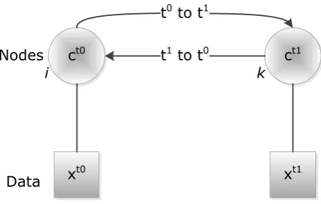
t0Figure 1. Designed CRF graph structure; node links are edges.
stationary transition matrix by Hoberg et al. (2015) as explained in subsequent sections.
Spatial-temporal CRF models posterior probability in Equation (2) with a graph structure where nodes are connected to image sites byA, I represent edges bearing relationships of adjacent sites
iand j in one epoch, and an additional potential, T P, repre-senting edges containing relationships between temporal sitesi
andkin different epochs as shown in Figure 1. In CRF frame-work,A,IandT Pcan be regraded as arbitrary local classifiers. This property enables use of domain-specific discriminative clas-sifiers in structured data rather than restricting the potentials to a certain form (Zhong and Wang, 2007a,b). We omit weight nota-tionsλ1andλ2in subsequent sections for clarity in CRF poten-tial equations.
2.3 Association Potential
It determines how likely an image siteitakes a labelct0 i in epoch site-wise feature vector (Kumar, 2006). We adopt random forest (RF) (Breiman, 2001) to determineAby independent classifica-tion of different epochs assuming class condiclassifica-tional independence in them. A RF conducts classification by casting votes from a number of decision treesDT generated during training. If the
number of votes cast for a given classcby RF isVc, then ourA value RF stabilizes (Hastie et al., 2011) and set tree depth as 25.
2.4 Interaction Potential
It measures the influence of data and neighbouring labels on site
iin epocht0. It ensures that sitei, as initially determined by association potential, is labelled to its corresponding ”true class” given data evidencext0
and neighbourhood dependencyNwhere
j∈N. This study modelsIusing contrast sensitive Potts model designed based on Euclidean distancedijof adjacent node
fea-turesfiandfj:
dij=
||fi(xt0)−fj(xt0)||
R (3)
whereRis the number of features. Then, model ofIis:
I(ct0
whereβis a spatial interaction parameter that regulates smooth-ness, parameter η regulates the contrast-sensitive term and
h(cti0, ct 0
j )is a histogram matrix count bearing co-occurrence of
labels of neighbouring sitesiandj. We normalize the histogram by row in order to minimize bias of dominant classes in train-ing data. Therefore, the model is different from contrast sensitive Potts model because transitions of classes is now governed by their frequency in training data (Kosov et al., 2013).
2.5 Temporal interaction potential
It models interactions between dataxt0
andxt1
We consider crop classification within one season. Consequently, spectral changes in classes at a given epoch are a result of phenol-ogy rather than transitions to other classes in another epoch. This is because a particular crop type is observed in the entire season from planting to harvest. We exploit the fact that crop phenology varies temporally and also spectrally to enhance crop discrimi-nation. Spectral changes due to crop phenology is expressed by joint probability in Equation (5).
Transitional probabilities between similar and different classes can be represented in a transitional matrixTik. The matrix can
be determined by expert opinion, empirically from existing data sources or computed (Liu et al., 2008). We computeTikfor each
site in the image using conditional probability computed from class membership probability vectors for nodeiandkestimated by RF for each site based on spectral observation in training sites. The matrix is then used to introduce a temporal directed edge between nodeiandkas illustrated in Figure 1.
2.5.1 Site-wise transition probability matrix Conditional probability expresses the likelihood of a class label to take up a siteiin epocht0given class label information from a sitek
in epocht1. It represents intra- and inter-class transitions. Con-sider a set of classesaandbsuch thatα∈ α1, α2, . . . , αaand
where prior probabilities P(ct0
i = α) and P(ct 1
k = ω) are
marginal distributions in Table 1. From rules of probability, sum rule
Equation (6) can be transformed into:
P(ctk1=ω|c
Therefore, from Equations (9) and (10) we compute site-wise transition probability matrix by dividing thea×bjoint proba-bility matrix of joint distributions in Table 1 by row sum and col-umn sum (marginal distributions) for crop phenology transitions int0⇒t1andt1⇒t0respectively.
2 3
ω1 ω2 . . . ωb Sum
ω1 P(α1, ω1) P(α1, ω2) P(α1, ωb) P(α1)
α2 P(α2, ω1) P(α2, ω2) P(α2, ωb) P(α2) ..
.
αa P(αa, ω1) P(αa, ω2) P(αa, ωb) P(αa)
Sum P(ω1) P(ω2) P(ωb) 1
Table 1. Computation of site-wise conditional probability matrix.
2.6 Training, Inference and parameter estimation
Solution to Equation (2) is obtained by maximizing probabilities, spectral(A), spatial(I)and temporal(T P)using Bayes’ Max-imum A Posterior (MAP) estimate. This requires an inference algorithm and we employ sum-product Loopy Belief Propaga-tion (LBP). The associaPropaga-tion potential probabilities used in bothI
andT Pare trained using RF implemented in OpenCV (OpenCV, 2014). We determineIparametersβandηwith help of Powell’s search method (Kramer, 2010) and setβ = 5andη = 1in all experiments. All potentials (A, I, andT P) were given an equal weight, i.e.λ1 =λ2 = 1.
3. Implementation
3.1 Study site and data
The study was conducted in northern Germany (52.26◦ N, 9.84◦
E) (Fig. 6). The region is characterized by intensive agri-culture, with large field sizes. The average annual precipitation in the area is 656 mm and the average annual temperature is8.9◦
C (January0.6◦
C, July17.5◦
C) (Deutscher Wetterdienst, 2012).
´
0 450
Km
Legend
study site agricultural areas
non agricultural areas
´
0 1 2 3 4
Kilometers
´
Figure 2. Location of the study site.
We use two dual polarized (HH and VV) TerraSAR-X High Res-olution Spotlight images acquired on 11th March 2009 and 18th June 2009 at an incidence angle of34.75◦
with a ground resolu-tion of 2.1 m in ground range direcresolu-tion and 2.4 m in azimuth direction. The images were delivered as ground range prod-ucts (MGD) with equidistant pixel spacing. All images are co-registered to an extent of 7.1×11.8km2
and projected to WGS 1984 UTM Zone 32N. Experiment site used covers an extent of 2.3×2km2
.
2P
(ct1 k =ω|ct
0 i =α) 3P
(ct0 i =α|ct
1 k =ω)
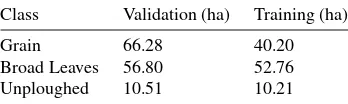
Ground reference data campaign was conducted concurrently with image acquisition. We divided ground reference polygons for separate use in training and validation as shown in Table 2. Separation of the ground reference polygons was done using stratified random sampling in sampling design tool in ArcGIS 10.0 (Buja and Menza., 2013).
Class Validation (ha) Training (ha)
Grain 66.28 40.20
Broad Leaves 56.80 52.76
Unploughed 10.51 10.21
Table 2. Data used for validation and training in hectares (ha).
3.2 Classes
The study area has the following crops:
1. Grain: oat, barley, wheat and rye,
2. Broad leaved (BL) crops: maize, potatoes, canola and sugar beets,
3. Unploughed (Unp): grassland, ruderal and hedges.
We adopt the three main classes for classification using our ap-proach in Equation (2).
The listed crops go through different phases at different times a fact that can enhance discrimination. A crop phenology calendar is shown in Figure 3. Four phases, preparation, seeding, growing, harvesting and post harvest, are considered. Preparation phase involves ploughing and soil grooming processes before seeding. In seeding phase, crop seeds are placed in the soil. Growing phase includes the period between crop germination to ripening. After ripening, harvesting starts where mature crops are gathered from the fields using relevant methods. The last stage is post harvest phase where the field could be fallow or with some remaining ripe crops.
Jan Feb Mar Apr May Jun Jul Aug Sep Oct Nov Dec
Maize
Pot at oes
Canola
Sugar beet s
Oat
Bar ley
Wheat
Rye
Unploughed
Jan Feb Mar Apr May Jun Jul Aug Sep Oct Nov Dec
Har vest ing Gr ow ing
Seeding
Pr eparat ion Post Har vest
Figure 3. Phenology stages of crops considered for classification.
3.3 Features
Classification using Equation (2) requires definition of site-wise feature vectorsfi(xt
0
)used in bothAandI. We compute eight texture features (mean, variance, homogeneity, contrast, dissimi-larity, entropy, second moment, and correlation) from Gray Level Co-occurrence Matrix (GLCM) (Haralick et al., 1973) using a 3×3window with0◦
direction. The features were computed from the dual polarized TerraSAR-X amplitude values in each epoch. Thusfi(xt
0
the distance function,dij, inIis a 16 dimensional feature vector,
i.e. R = 16in Equation (3). All the features were normalized between 0 and 1 to minimize undue influence by features with high values.
3.4 Experiments
To evaluate our approach we conducted experiments using the test site and data described in Section 3.1. The experiments were done using fourapproaches:
3.4.1 Approach 1 In this approach we use RF in Section 2.3 for mono-temporal classification of crops. Approach 1 also forms
Ain CRF.
3.4.2 Approach 2 experiments are based on mono-temporal CRF in Section 2.1. Basically, it considers spatial context only with no temporal interactions hence ”mono-temporal”.
3.4.3 Approach 3 is an existing state-of-the-art spatial-temporal MRF approach in (Liu et al., 2008). We implement this approach for comparison with spatial-temporal CRF devel-oped in the study. In the approach, site-wise transitional matrix were determined using conditional probabilities described in Sec-tion 2.5.1. To implement spatial-temporal MRF we setη= 0in Equation (2) but, other parameters remain as described in Sec-tion 2.6. This eliminates data interacSec-tion inI reducing it to a MRF Ising model:
3.4.4 Approach 4 is the spatial-temporal CRF approach pre-sented in this paper, where the site-wise transition matrix is com-puted from conditional probabilities as shown in Section 2.5.1. The approach is an extension of MRF forest change detection method in (Liu et al., 2008) into CRF crop type classification us-ing crop phenology informattion.
3.5 Results
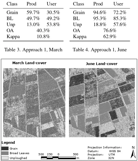
In conducted experiments, we applied cross-validation based on reference data in Table 2 to evaluate our approach (approach 4) vis-`a-vis approaches 1 to 3 in Section 3.4. Overall accuracy (OA), kappa statistic, producer (Prod) and user (User) accuracy mea-sures were computed from error matrices generated by comparing classified pixels against validation set. These accuracy measures are illustrated in Tables 3 to 10.
Tables 3 and 4 illustrate results of approach 1, RF, in both epochs (June and March). Approach 1 considers no spatial-temporal in-formation and thus accuracy values are low. Classification accu-racy is particularly low in March with many pixels mislabeled as
shown in Figure 4 compared to June. This is because of different phenological states of crops as demonstrated in Figure 3.
Class Prod User
Table 3. Approach 1, March
Class Prod User
Table 4. Approach 1, June
March Land-cover June Land-cover
Legend
Figure 4. Approach 1, RF, classification used as baseline.
Introduction of spatial interaction by approach 2 using CRF im-proves discrimination of crops as shown in Tables 5 and 6. The OA improves by 3.2% and 11.7% in March and June respectively.
Class Prod User
Table 5. Approach 2, March
Class Prod User
Table 6. Approach 2, June
Results of addition of temporal potential using approach 3 in (Liu et al., 2008) are shown in Tables 7 and 8. Approach 3 improved classification OA by 48% and 12.8% in march and june when compared to approach 1 in Tables 5 and 6. In comparison to approach 2 OA improved by 45.1% and 1.1% in march and june respectively. This depicts importance of temporal information.
Class Prod User
Table 7. Approach 3, March
Class Prod User
Table 8. Approach 3, June
compared to CRF mono-temporal classification in Tables 5 and 6 considering classification accuracy improved by 47.3% and 2.9% in March and June respectively. In comparison with approach 3, MRF spatial-temporal classification, approach still improved OA by 2.5% and 1.8% in march and june respectively.
Class Prod User
Grain 97.5% 91.0%
BL 94.9% 94.9%
Unp 47.2% 67.1%
OA 90.8%
Kappa 84.1%
Table 9. Approach 4, March
Class Prod User
Grain 94.2% 94.7%
BL 96.2% 95.1%
Unp 46.7% 47.8%
OA 91.2%
Kappa 84.5%
Table 10. Approach 4, June
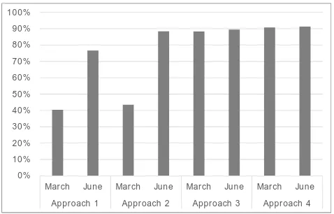
A comparison of performance of all methods using OA is de-picted in Figure 5. The diagram shows that approach 4 generally performs well in both epochs compared to other approaches.
0% 10% 20% 30% 40% 50% 60% 70% 80% 90% 100%
March June March June March June March June Approach 1 Approach 2 Approach 3 Approach 4
Figure 5. Overall accuracy summary of all approaches.
March Land-cover June Land-cover
Legend
Grain Broad Leaves
Unploughed
±
Projection Information: Datum: WGS 84 Projection: UTM Zone 32N 500 250 0 500
m
Figure 6. Land-cover maps produced using approach 4.
4. Discussion
The aim of this study was to design a spatial-temporal approach that exploits phenological changes within a vegetation season to improve discrimination of crops. Random forest, approach 1, used inAof CRF considers pixel-wise labelling by voting us-ing decision trees. Results of this approach are characterized by mislabeled pixels in the form of ”salt and pepper” as shown in Figure 4 which impacts classification accuracy. This illustrates
significance of context in classification. We used RF as a base-line to incorporate spatial and temporal context using CRF.
As demonstrated in Tables 5 and 6, spatial interaction introduced by CRF significantly improved crop discrimination. The CRF interaction potential models site dependencies in a statistically sound manner in order to allocate a label to a given site. This min-imizes ”salt and pepper” effect common in per pixel approaches by ensuring that sites are labelled in regard to neighbouring labels and data.
Addition of temporal term further enhanced crop discrimination by exploiting crop phenology. Phenology enhanced class dis-crimination because different crops vary spectrally in time. For instance, the unploughed group of crops grow throughout the year, Figure 3, and has higher accuracy in june when other crops are in growing stage. Its spectral discrimination reduces later in march when most crops are in preparation stage because they are covered by similar land-cover. We incorporated this knowledge intoT Pfor classification using approaches 3 and 4.
Results from approach 3 and 4 indicate an increase in clas-sification accuracy. The two approaches use site-wise condi-tional probabilities to compute temporal transition matrix. Condi-tional probabilities determine probability of inter- and intra-class changes. During a vegetation season, observed spectral changes are only within a class. Therefore, transition from classAto an-other classBare minimal assuming no natural or artificial crop interference. We use this fact to enhance discrimination of classes that can not be separated easily, for instance in march epoch. However, approach 3 is based on MRF which ignores spatial in-teractions in data a fact that makes it perform lower than CRF. We therefore implemented the approach in CRF, i.e. approach 4.
Observations from approach 3 led us to design a robust method (approach 4) to incorporate phenology information in all epochs. We use site-wise conditional probability to compute temporal transition matrix. So far our approach demonstrates stable accu-racy in considered epochs. This is because conditional probabil-ity facilitate bi-directional exchange of temporal information in form of probabilities thereby enhancing accuracy of a class with low discrimination in either epoch. The approach is suitable for seasonal crop classification since uncertainty in a class at a given epoch is resolved in another. For instance, low accuracy in grain and broad leaved classes in March, see Table 3, is improved by our approach as shown in Table 9. Moreover, our temporal term (T P) is data dependent unlike in (Hoberg et al., 2015) where it was determined by empirically.
5. Conclusion and outlook
Our study has demonstrated significance of spatial-temporal in-formation for seasonal crop classification. Spatial interaction sig-nificantly enhances spatial dependency minimizing ”salt and pep-per” effect common in per pixel classifiers. The introduced tem-poral potential resolved classes with low accuracy in March 2009 using information from June 2009 based on crop phenological changes in time. Moreover, our approach outperforms existing MRF state-of-the art spatial-temporal approach. Follow up stud-ies will consider classification of sub-categorstud-ies of crops and us-ing images acquired at more than two epochs.
ACKNOWLEDGEMENTS
References
Bargiel, D., Herrmann, S., Lohmann, P. and S¨orgel, U., 2010. Land use classification with high-resolution satellite radar for estimating the impacts of land use change on the quality of ecosystem services. In:ISPRS TC VII Symposium: 100 Years ISPRS, Vol. XXXVIII, IAPRS, Vienna, Austria, pp. 68–73.
Breiman, L., 2001. Random forests. Machine Learning45(1), pp. 5–32.
Buja, K. and Menza., C., 2013. Sampling Design Tool for ArcGIS - Instruction Manual. NOAA, Silver Spring, MD.
Deutscher Wetterdienst, 2012. Mittelwerte der Temperatur und des Niederschlags bezogen auf den aktuellen Standort. Online: http://www.dwd.de.
Geman, S. and Geman, D., 1984. Stochastic Relaxation, Gibbs Distributions, and the Bayesian Restoration of Images. IEEE Transactions on Pattern Analysis and Machine Intelligence
PAMI-6(6), pp. 721–741.
Gomez-Chova, L., Fern´andez-Prieto, D., Calpe, J., Soria, E., Vila, J. and Camps-Valls, G., 2006. Urban monitoring using multi-temporal SAR and multi-spectral data.Pattern Recogni-tion Letters27(4), pp. 234–243.
Goodchild, M. F., 1992. Geographical information science. In-ternational Journal of Geographical Information Systems6(1), pp. 31–45.
Gould, S., Rodgers, J., Cohen, D., Elidan, G. and Koller, D., 2008. Multi-class segmentation with relative location prior.
International Journal of Computer Vision80(3), pp. 300–316.
Haralick, R. M., Shanmugam, K. and Dinstein, I., 1973. Textu-ral Features for Image Classification. IEEE Transactions on Systems Man and Cybernetics3(6), pp. 610–621.
Hastie, T., Tibshirani, R. and Friedman, J., 2011.The Elements of Statistical Learning: Data Mining, Inference, and Prediction. Springer Series in Statistics, 2nd edn, Springer.
He, W., J¨ager, M., Reigber, A. and Hellwich, O., 2008. Build-ing Extraction from Polarimetric SAR Data usBuild-ing Mean Shift and Conditional Random Fields. In:EUSAR, Friedrichshafen, Germany, pp. 1–4.
He, X., Zemel, R. and Carreira-Perpi˜n´an, M., 2004. Multiscale conditional random fields for image labeling. In:CVPR, Vol. 2, Washington, DC, USA, pp. 695–702.
Hoberg, T. and M¨uller, S., 2011. Multitemporal Crop Type Classification Using Conditional Random Fields and Rapid-Eye Data. In:ISPRS, Hannover, Germany.
Hoberg, T. and Rottensteiner, F., 2010. Classification of settle-ment areas in remote sensing imagery using conditional ran-dom fields. In: ISPRS TC VII Symposium-100 Years ISPRS, Vienna, Austria.
Hoberg, T., Rottensteiner, F. and Heipke, C., 2010. Classifica-tion of multitemporal remote sensing data using CondiClassifica-tional Random Fields. In:IAPR Workshop on Pattern Recognition in Remote Sensing, pp. 1–4.
Hoberg, T., Rottensteiner, F. and Heipke, C., 2011. Classification of multitemporal remote sensing data of different resolution using Conditional Random Fields. In:ICCV, pp. 235–242.
Hoberg, T., Rottensteiner, F., Feitosa, R. and Heipke, C., 2015. Conditional Random Fields for Multitemporal and Multiscale Classification of Optical Satellite Imagery.IEEE Transactions on Geoscience and Remote Sensing53(2), pp. 659–673.
Jeon, B. and Landgrebe, D., 1992. Classification with spatio-temporal interpixel class dependency contexts.IEEE Transac-tions on Geoscience and Remote Sensing30(4), pp. 663–672.
Jianya, G., Haigang, S., Guorui, M. and Qiming, Z., 2008. A review of multi-temporal remote sensing data change de-tection algorithms. The International Archives of the Pho-togrammetry, Remote Sensing and Spatial Information Sci-encesXXXVII(B7), pp. 757–762.
Kenduiywo, B. K., Tolpekin, V. A. and Stein, A., 2014. Detection of built-up area in optical and synthetic aperture radar images using conditional random fields. Journal of Applied Remote Sensing8(1), pp. 083672–1 – 083672–18.
Korc, F. and F¨orstner, W., 2008. Interpreting terrestrial images of urban scenes using discriminative random fields. In: ISPRS, Beijing, China, pp. 291–296.
Kosov, S., Kohli, P., Rottensteiner, F. and Heipke, C., 2013. A two-layer conditional random field for the classification of par-tially occluded objects.ArXiv e-prints.
Kramer, O., 2010. Iterated local search with Powell’s method: a memetic algorithm for continuous global optimization.
Memetic Computing2(1), pp. 69–83.
Kumar, S., 2006. Discriminative random fields. International Journal of Computer Vision68(2), pp. 179–201.
Lafferty, J. D., McCallum, A. and Pereira, F., 2001. Conditional random fields: probabilistic models for segmenting and label-ing sequence data. In: ICML, Morgan Kaufmann, San Fran-cisco, CA, USA, pp. 282–289.
Leite, P., Feitosa, R., Formaggio, A., da Costa, G., Pakzad, K. and Sanches, I., 2011. Hidden Markov Models for crop recog-nition in remote sensing image sequences.Pattern Recognition Letters32(1), pp. 19–26.
Li, S. Z., 2009. Markov random field modeling in image analy-sis. Advances in pattern recognition, 3rd edn, Springer-Verlag, London.
Liu, D., K., S., Townshend, J. and Gong, P., 2008. Using local transition probability models in markov random fields for for-est change detection. Remote Sensing of Environment112(5), pp. 2222 – 2231.
Liu, D., Kelly, M. and Gong, P., 2006. A spatial-temporal approach to monitoring forest disease spread using multi-temporal high spatial resolution imagery. Remote Sensing of Environment101(2), pp. 167–180.
Lu, D. and Weng, Q., 2007. A survey of image classifica-tion methods and techniques for improving classificaclassifica-tion per-formance. International Journal of Remote Sensing 28(5), pp. 823–870.
Melgani, F. and Serpico, S., 2003. A Markov random field approach to spatio-temporal contextual image classification.
IEEE Transactions on Geoscience and Remote Sensing41(11), pp. 2478–2487.
Moser, G. and Serpico, S., 2011. Multitemporal region-based classification of high-resolution images by markov random fields and multiscale segmentation. In: IGARSS, Vancouver, Canada, pp. 102–105.
Niemeyer, J., Rottensteiner, F. and S¨orgel, U., 2013. Classifica-tion of urban LiDAR data using condiClassifica-tional random field and random forests. In:JURSE, pp. 139–142.
Niemeyer, J., Wegner, J. D., Mallet, C., Rottensteiner, F. and S¨oergel, U., 2011. Conditional random fields for urban scene classification with full waveform lidar data. In: Photogram-metric Image Analysis, Springer, pp. 233–244.
OpenCV, 2014. Random Trees. http://docs.opencv.org/ modules/ml/doc/ml.html. [Accessed: 20-11-2014]. Parikh, D. and Batra, D., 2008. CRFs for image classification.
Technical report, Carnegie Mellon University.
Solberg, A. H. S., Taxt, T. and Jain, A., 1996. A markov random field model for classification of multisource satellite imagery.
IEEE Transactions on Geoscience and Remote Sensing34(1), pp. 100–113.
Swain, P. H., 1978. Bayesian Classification in a Time-Varying Environment.IEEE Transactions on Systems, Man and Cyber-netics8(12), pp. 879–883.
Tso, B. and Mather, P. M., 2009. Classification methods for re-motely sensed data. 2nd edn, CRC Press, Boca Raton.
Tupin, F., 2010. Fusion of Optical and SAR Images. In: U. S¨orgel (ed.),Radar Remote Sensing of Urban Areas, Remote Sensing and Digital Image Processing, Vol. 15, Springer, Netherlands, pp. 133–159.
Wegner, J., H¨ansch, R., Thiele, A. and S¨orgel, U., 2011a. Build-ing Detection From One Orthophoto and High-Resolution In-SAR Data Using Conditional Random Fields. IEEE Journal of Selected Topics in Applied Earth Observations and Remote Sensing4(1), pp. 83–91.
Wegner, J., S¨oergel, U. and Rosenhahn, B., 2011b. Segment-based building detection with conditional random fields. In:
JURSE, Munich, Germany.
Zhong, P. and Wang, R., 2007a. A multiple conditional random fields ensemble model for urban area detection in remote sens-ing optical images.IEEE Transactions on Geoscience and Re-mote Sensing45(12), pp. 3978–3988.