GENERATION OF THE AUSTRALIAN GEOGRAPHIC REFERENCE IMAGE
THROUGH LONG-STRIP ALOS PRISM ORIENTATION
M. Ravanbakhsh a, L.-W. Wang b, C.S.Fraser a, *, A. Lewis b
a
CRC for Spatial Information, Box 672, Carlton Sth, Vic 3053, Australia - (m.ravanbakhsh, c.fraser)@unimelb.edu.au b
Geoscience Australia, GPO Box 378, Canberra, ACT 2601, Australia - (lan-wei.wang, adam.lewis)@ga.gov.au
Commission I, WG I/4
KEY WORDS: satellite imagery, georeferencing, ALOS PRISM, orthorectification, long-strip adjustment
ABSTRACT:
The Australian Geographic Reference Image (AGRI) is a national satellite image mosaic that covers the vast Australian continent. Formed from 9560 ALOS PRISM images, AGRI provides a spatially correct reference image at 2.5m resolution, with 1-pixel accuracy. The production of AGRI was made feasible by the development and implementation of a long-strip adjustment technique that facilitated a refinement in the georeferencing process of orbit and attitude parameters for orbital segments comprising 50 or more images. The strip of images is effectively treated as a single image. The ground control requirements for such full-pass georeferencing, which does not require the measurement of tie or pass points, amount to only 4-8 GCPs for the complete strip rather than 4 or more per image within the strip. Once the adjusted orbit parameters are obtained, the georeferencing and orthorectification process can revert to a fully automatic image-by-image computation. This paper first overviews AGRI and then describes the long-strip adjustment technique that made its production possible. Testing and validation are then discussed via the example of the georeferencing of a 1527km single strip of 55 PRISM images. The testing phase verified that 1-pixel accuracy georeferencing could be achieved with the long-strip adjustment approach, and in the production of AGRI accuracy checks against 2460 checkpoints yielded an RMS discrepancy of close to 2.5m and a 90% Circular Error (CEP90) of 5.5m.
* Corresponding author.
1. INTRODUCTION
With the advent of high-resolution satellite imagery, accurate georeferencing has assumed greater importance for a number of remote sensing applications. Consistency and accuracy in broad-area image orthorectification is essential to ensure that observations taken at different times, from different sources can be compared at single-pixel resolution, thus allowing temporal monitoring where each pixel can be compared 'with itself' through time. The georeferencing operation has traditionally required ground control points (GCPs) that support image-by-image orthorectification. A more recent approach involves the provision of a single controlled image base, formed by a mosaic of orthorectified high-resolution satellite images. Individual satellite images can then be georeferenced automatically to this ‘reference image’ through image matching, thus alleviating the subsequent need for GCPs.
For a country the size of Australia, provision of a reference image formed by orthorectified ALOS PRISM imagery of 2.5m resolution, in a scene-by-scene rectification process, would constitute a daunting task, with some 6,000 PRISM OB1 scenes (35km x 35km) in nominally 110 orbital passes being required to cover a land area of 7.6 million km2. The number of GCPs needed would be 30,000 or so. Yet, the planned Australian Geographic Reference Image was to be produced from PRISM imagery and thus a new photogrammetric data processing approach was needed to realise the production of such a country-wide reference image. The approach developed, namely georeferencing through the adjustment of very long strips of imagery, forms the topic of this paper.
2. AUSTRALIAN GEOGRAPHIC REFERENCE IMAGE
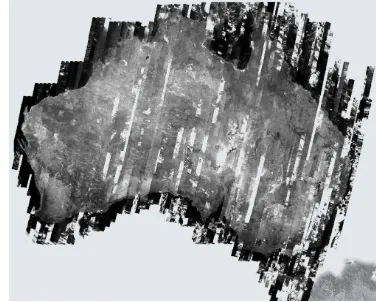
Illustrated in Figure 1 is the Australian Geographic Reference Image (AGRI), which was produced by Geoscience Australia (GA). AGRI is a national mosaic of orthorectified ALOS PRISM image strips covering the entire Australian continent. It provides an accurate positional reference system for satellite imagery with spatial resolutions of 2.5m or less.
Figure 1. AGRI national mosaic of ALOS PRISM imagery.
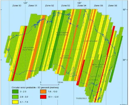
AGRI was formed through a mosaicking of 9560 images from 206 strips of PRISM OB1- and OB2-mode images, some covering the full north-south span of the continent and others comprising strip segments of various lengths. Full details of the production process are provided in Lewis et al. (2011). The stages of the process comprised selection of imagery from GA’s
ALOS archive, collection of the required GCPs, georeferencing of the imagery to nominally 1-pixel accuracy, generating the orthoimagery and building the orthoimage mosaic.
The topic of this paper is the georeferencing of PRISM imagery, and specifically the long-strip adjustment technique that was primarily developed to support the AGRI initiative. In the absence of corrections for positional and attitude biases in the orbital data provided with ALOS imagery, GA could provide a georeferencing accuracy for PRISM images of no better than 15m. Accuracy can be readily increased to 1-pixel level (2.5m) through the provision of ground control, but as has already been mentioned, some 30,000 GCPs would be needed to perform a scene-wise georeferencing. The long-strip adjustment technique drastically reduced the number of required GCPs and made achievable an otherwise infeasible task.
Figure 2. 206 PRISM image strips used to compile AGRI, along with estimates of strip georeferencing accuracy.
3. LONG-STRIP ADJUSTMENT AND GEOREFERENCING
3.1 Overview
The method of long-strip adjustment for orientation and georeferencing of PRISM imagery, first reported in Rottensteiner et al. (2008, 2009) and Weser et al. (2008a,b), is based on the merging of successive images within a single satellite pass into what amounts to a single image covering the entire orbit segment. Metadata for each separate scene is merged to produce a single, continuous set of orbit and attitude parameters, such that the entire strip of tens of images can be treated as a single image, even though the separate scenes are not actually merged. Within the strip adjustment, the orbit parameters are refined based on the provision of GCPs at each end of the strip. The approach differs from currently employed strip and block adjustment approaches for high-resolution satellite imagery that utilise physical sensor models (eg Chen et al., 2006; Toutin, 2006; Crespi et al., 2007; Poli, 2007) in that there is no requirement to measure pass/tie points within the imagery. The only image measurements needed are to the relatively few GCPs, which are generally positioned at each end of the strip.
As described in Fraser & Ravanbakhsh (2011), a minimum of four GCPs is required to achieve 1-pixel georeferencing
accuracy for PRISM strips, even for strip lengths of 1000 km or more. The merging of orbit data results in a very considerable reduction in both the number of unknown orientation parameters and the number of required GCPs in the sensor orientation adjustment. Indeed the number of required GCPs can drop from well over 100 to only 4-6 for a 50-image orbit segment.
The reported strip adjustment approach makes use of a generic sensor orientation model. However, the parameters of this model are not necessarily conducive to exploitation by standard photogrammetric workstations. Thus, in order to further photogrammetrically process imagery forming the adjusted strip, RPCs can be generated for each intermediate image from the adjusted sensor orientation. The RPCs then facilitate bias-free georeferencing in any scene without reference to ground control.
3.2 Sensor Orientation Model
Only a brief description of the sensor orientation model used for the long-strip adjustment will be provided here; full details are provided in Weser et al. (2008a;b). The physical model for a pushbroom satellite imaging sensor relates a point PECS = (XECS,
YECS, ZECS)T in an earth-centered object coordinate system to
the position of its projection pI = (xI, yI,0) T
in an image coordinate system. The coordinate yI of an observed image
point directly corresponds with the recording time t for the image row through t = t0 + ∆t · yI, where t0 is the time of the
first recorded row and ∆t the time interval between scans. The framelet coordinate system, in which the observation pI can be
expressed as pF = (xF, yF, zF)T = (xI, 0, 0)T, refers to an
individual CCD array. The relationship between an observed image point pF and the object point PECS is given as
pF=cF + µ · RM T
· {RP T
(t) · RO T
· [PECS – S(t)] – CM}–δδδδx (1)
Here, cF = (xFC, yFC, f) describes the interior orientation, ie the
position of the projection centre in the framelet coordinate system. The vector x formally describes corrections for systematic errors such as velocity aberration and atmospheric refraction. The shift CM and the rotation matrix RM describe a
rigid motion of the camera with respect to the satellite. They are referred to as the camera mounting parameters.
The satellite orbit path is modelled by time-dependent functions, ie S(t)=[X(t),Y(t),Z(t)]T, and the sensor attitudes are described by a concatenation of a time-constant rotation matrix RO and a matrix RP(t). These are parameterized by
time-dependant functions describing three rotation angles, roll(t), pitch(t) and yaw(t). The components of the orbit path and the time-dependant rotation angles are in turn modelled by cubic spline functions. The rotation matrix RO rotates from the
earth-centred coordinate system to one that is nearly parallel to the satellite orbit path and this matrix can be computed from the satellite position and velocity at the scene centre.
3.3 The PRISM Sensor
A feature of ALOS PRISM is that depending on the imaging mode, four or six CCD arrays are used to record a scene, each array producing a separate image file. These sub-images share the same exterior orientation, camera mounting parameters and focal length. However, each has its own framelet coordinate system, so the coordinates of the principal point can be different for each (see Weser et al., 2008b). In order to treat the
images as a single image, a correction vector δδδδx = (δx, δy, 0)T is used. The interior orientation parameters cF = (xFC, yFC, f) are
assumed to be identical for all sub-scenes, with corrections (δxi,
δyi) for the relative misalignment of the CCD chips then
offsets a0 and b0 model the different positions of the origins of
the individual framelet coordinate systems relative to the camera coordinate system, and a1i and b1i correct for small
perturbations in the pixel sizes of the CCD arrays with respect to each other. The parameter b2i models any deviation of the
CCD array from a straight line, whereas a2i is related to
non-linear variations in pixel size. The required sensor orientation model for ALOS PRISM is formed through a substitution of Eq. 2 into Eq. 1.
3.4 Strip Adjustment
Refined estimates of the parameters of the sensor model are achieved through bundle adjustment of the strip(s) of imagery. The observations comprise the framelet coordinates of image points (both control points and tie points in the case of multiple strips), the corresponding object coordinates of GCPs, and direct observations for the orbit path and attitudes derived from the metadata. Systematic errors in the direct observations of orbit path and attitude are modeled by expanding the associated cubic spline functions so that for each orbit observation pobs at systematic error correction parameters per satellite orbit, namely three offsets ( X, Y, Z)T for the orbit path points and three offsets ( roll, pitch, yaw)T for the rotation angles, are
determined along with the spline parameters.
For stereo and 3-line PRISM imaging configurations, or for overlapping strips of imagery, bundle adjustment can directly yield 3D ground point coordinates from the corresponding observed image point pairs or triplets. In the case of a single strip of near nadir scenes, however, only a single set of image coordinates can be measured for the corresponding ground point. The term bundle adjustment is thus a little misleading since no direct computation of the ground coordinates of any measured image point can be performed within the adjustment. Instead, the process is effectively one of spatial resection from GCPs in which exterior orientation parameters are refined. Only the single-strip case will be considered here.
The first step in the long-strip adjustment process involves an initial merging of scenes along with their associated orbit and attitude data. A single set of camera mounting and interior orientation parameters then applies for the orientation of what may now be considered a single composite image. Also, the six bias correction parameters for orbit path and attitude relate to the entire strip. The resulting adjusted orientation and bias-correction parameters for the strip can then be mapped back to the individual scenes to refine their orientation.
3.5 Scene Georeferencing and Orthoimage Generation
The strip adjustment provides a bias correction within the sensor orbit and attitude data and the adjusted exterior orientation can be delivered to the user in the form of newly generated, bias-corrected RPCs. Georeferencing can then follow as a separate rather than integral part of the strip adjustment process. The RPC model, as computed using camera and sensor orientation parameters, is universally accepted as a valid alternative sensor orientation model for High Resolution Satellite Imagery (eg Fraser et al., 2006). RPCs facilitate the transformation from image to object space coordinates and in the case of the production of AGRI they were employed for the orthorectification process, the underlying elevation model being the 1-second DEM from the Shuttle Radar Topography Mission (SRTM).
The actual mosaicking process employed for AGRI involved the individual orthorectified images within a strip segment first being combined to form ‘pass images’. These 206 pass images were then intensity and contrast balanced before being formed into seven separate UTM zone mosaics with 2.5m resolution. A single continental mosaic at 0.0001 deg. (approx. 10m) resolution was also produced (Lewis et al., 2011).
4. EXPERIMENTAL TESTING
4.1 Scope
A number of experimental tests were conducted of the long-strip adjustment process for PRISM imagery, both by GA and by the CRC for Spatial Information. GA utilised the Barista software (Barista, 2012) system incorporating the long-strip adjustment approach on two pass segments, one 2000km in length and the other of 730km length. In the longer strip a small number of GCPs were positioned at the top, middle and bottom, whereas they were located only in the middle and bottom of the shorter strip. As detailed in Lewis et al. (2011), checkpoint accuracy was around 1 pixel (2.5m) RMS across track and 1.4 pixel (3.5m) along track. Notable in the results of the shorter strip was that accuracy of better than 2 pixels (5m) was obtained at the extremity of the segment where the strip extended beyond the GCPs by as much as 20 scenes. This was seen as very positive in the context of using the method to georeference offshore islands.
The scope of testing at the CRC for Spatial Information covered two long-strip data sets of PRISM nadir imagery, with the data processing commencing with the importing of images and associated metadata into Barista. A merging of the recorded orbit and attitude data for the strip(s) then takes place. This is followed by the collection of ground points, these being GCPs as well as check points, and the subsequent measurement of image coordinates. Next, strip adjustment is performed using a small number of GCPs, and checkpoint discrepancies (residuals) are computed in image space via back projection utilising the adjusted (and bias corrected) exterior orientation for each image. Monoplotting is then employed to assess the planimetric accuracy in object space. Finally, RPCs are generated for each scene from the adjusted orbit orientation parameters, and the same accuracy evaluation in both image and object space is again performed to validate the computation of the RPCs. Provided that the RPCs model the adjusted sensor orientation data to an accuracy of better than 0.1 pixel, the (2)
results of the initial and final accuracy assessment should correspond for all practical purposes
The first data set to be evaluated comprised two 1760 km overlapping ALOS PRISM OB2 70km wide strips over Western Australia. This block comprised 124 scenes, each with 6 adjacent sub-scenes (separate CCD arrays), covering an area of 40 km in length and 70 km in width. The side overlap between the strips amounted to 25% percent. The only available sources of reference data for determination of 3D coordinates of GCPs over the whole 215,000 km2 area of the block were orthophotos and DEMs. The ground points derived from orthophotos were assigned height values by bilinear interpolation from the DEMs. Of the 100 points obtained, six were used as GCPs, located at the northern and southern end of the block, and the rest served as check points. The positional accuracy of the points was modest, being between 5 m and 10 m, with the height data having been derived from the 1-second SRTM DEM. Results from this 2-strip adjustment are detailed in Fraser & Ravanbakhsh (2011); here it is mentioned only that accuracy at the 1.1 pixel level in monoplotted 2D ground point coordinates was achieved with little difference between discrepancies along- and across-track.
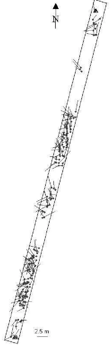
The second data set comprised a 1527 km long, 35km wide strip of 55 OB1 images from the same orbit over Eastern Australia, as shown in Figure 3. Each scene comprised sub-images from four CCD arrays. A total of 194 ground points were employed, either as GCPs or check points. Figure 3 indicates their location within the strip. The majority of the ground points were GPS-surveyed to 1m or better accuracy in planimetry and height. Some 19 points were determined using existing orthophotos and DEMs of the areas where more accurate reference data was not available. These points were distributed across the 17 northern-most scenes.
4.2 Results for 55-Image Strip
Long-strip adjustments were initially performed utilising two basic GCP configurations. In the first of these, GCPs were confined to the end and middle regions of the strip, and in the second to the end regions only. The outcome of this initial examination of GCP layout and location was that there was no requirement from an accuracy standpoint for the mid-strip GCPs and that optimal accuracy was attainable from as few as 2 – 3 GCPs at each end of the 1500 km strip. For the 55-image single strip, the GCP layout comprised two GPS-surveyed points at the southern end and two points derived from aerial orthoimagery and DEM data at the Northern end, as indicated by the point locations shown in Figure 3. The rest of the points are treated as check points, and since there was overlap between successive scenes, some check points appear twice.
The RMS values of checkpoint discrepancies in image space obtained from both the adjusted orbit data computed in the long-strip adjustment, and from application of the subsequently generated RPCs, are listed in Table 1. The corresponding values in object space, in UTM coordinates, are listed in Table 2 and the discrepancy vectors obtained through monoplotting are shown in Figure 3. Although 1-pixel across-track accuracy was achieved, the RMS error in the along-track direction reached 1.6 pixels or 3.9m. The cause of this larger error is thought attributable to the GCPs/checkpoints being of inhomogeneous accuracy, 19 having been determined from orthoimagery and DEM information.
5. CONCLUDING REMARKS
The results of the testing at both GA and the CRC for Spatial Information provided the necessary validation of the long-strip adjustment technique as a practical basis for the georeferencing of the PRISM image strips that would form AGRI.
An extensive ground survey operation was thus undertaken to establish some 2880 GPS-surveyed GCPs and checkpoints, essentially around the 12,000km perimeter and in a strip across the middle of mainland Australia (see Lewis et al., 2011), as well as in Tasmania. These GCPs then supported the long-strip georeferencing of 105 orbit segments, comprising a total of 9560 scenes. Accuracy checks against 2460 checkpoints showed an RMS discrepancy of close to 1 pixel and a 90% Circular Error (CEP90) of 5.5m. Visual checks were also made between the final AGRI mosaic and GPS tracking data, such as along roads.
Table 1. RMS values of checkpoint discrepancies x and y in image space coordinates, in pixels, for the 55-scene strip.
Table 2. RMS values of checkpoint discrepancies E and N in object space UTM coordinates, in metres, obtained via monoplotting with either adjusted orbit observations or the generated RPCs.
The AGRI concept has now been fully realised and this national image mosaic provides a new source of ground control across Australia. A consistent base image is an important foundation for future mapping and monitoring. AGRI was needed because imagery from emerging new satellites can be automatically registered to it, consistently and accurately. AGRI was made possible by the developed long-strip adjustment approach to satellite image georeferencing. This technique, implemented in Barista, rendered the project feasible in time, logistics and cost. It reduced the image registration problem from correction of almost 10,000 scenes to correction of just 206 orbit segments. Moreover, the number of required GCPs was reduced from more than 30,000 to less than 1000.
6. ACKNOWLEDGEMENTS
Figure 3. 55-scene, 1527km-long PRISM strip showing 4 GCPs (triangles) and discrepancy vectors in planimetry at 194 check points.
7. REFERENCES
Barista, 2012. Barista product information webpage, http://www.baristasoftware.com.au [last date accessed: 3 Apr. 2012].
Chen, L-C., Teo, T.-A. & Liu, C.-L., 2006. The Geometrical Comparisons of RSM and RFM for FORMOSAT-2 Satellite Images. Photogrammetric Engineering & Remote Sensing, 72(5), pp. 573-579.
Crespi, M., Fratarcangelli, F., Gianonne, F. & Pieralice,F., 2007. SISAR: a rigorous orientation model for synchronous and asynchronous pushbroom sensor imagery. International Archives of Photogrammetry, Remote Sensing and Spatial Information Sciences, 36(1/W51), 6 pages (on CD-ROM).
Fraser, C. S., Dial, G., Grodecki, J., 2006. Sensor orientation via RPCs. ISPRS Jnl Photogramm. & Remote Sens. 60(3), pp.182-194.
Fraser, C. S. & Ravanbakhsh, M., 2011. Precise Georeferencing of Long Strips of ALOS Imagery. Photogrammetric Engineering & Remote Sensing, 77(1), pp. 87-93.
Lewis, A., Wang, L-W. & Coghlan, R., 2011. AGRI: The Australian Geographic Reference Image. Technical Report GeoCat# 72657, Geoscience Australia, 37 pages. www.ga.gov.au/image_cache/GA20164.pdf
Poli, D., 2007. A rigorous model for spaceborne linear array sensor. Photogrammetric Engineering & Remote Sensing, 73(2), pp. 187-196.
Rottensteiner, F., Weser, T. & Fraser, C.S., 2008. Georeferencing and orthoimage generation from long strips of ALOS imagery. Proceedings of 2nd ALOS PI Symposium, ESA/JAXA, Rhodes, Greece, 3-7 Nov., 8 pages (on CDROM).
Rottensteiner, F., Weser, T., Lewis, A. & Fraser, C.S., 2009. A strip adjustment approach for precise georeferencing of ALOS imagery. IEEE Transactions on Geoscience & Remote Sensing, 47 (12; Part I), pp. 4083-4091.
Toutin, T., 2006. Spatiotriangualtion with multisensory HR stereo images. IEEE Transactions on Geoscience & Remote Sensing, 44(2), pp. 456-462.
Weser, T., Rottensteiner, F., Willneff, J., Poon, J. & Fraser, C. S., 2008a. Development and testing of a generic sensor model for high-resolution satellite imagery. Photogrammetric Record, 21(123), pp. 255-274.
Weser, T., Rottensteiner, F., Willneff, J. & Fraser, C. S., 2008b. An improved pushbroom scanner model for precise georeferencing of ALOS PRISM imagery. Intern. Arch. Photogrammetry, Remote Sensing & Spatial Information Sci., Beijing, XXXVII (B1-2), pp. 723-730.