TOWARDS A SEMANTIC INTERPRETATION OF URBAN AREAS WITH AIRBORNE
SYNTHETIC APERTURE RADAR TOMOGRAPHY
O. D’Hondt, S. Guillaso, O. Hellwich
Technische Universit¨at Berlin, Computer Vision & Remote Sensing, Sekr. MAR 6-5, Marchstr. 23, D-10587 Berlin (olivier.dhondt, stephane.guillaso, olaf.hellwich)@tu-berlin.de
KEY WORDS:Synthetic Aperture Radar, Tomography, Segmentation, Point Cloud, 3D.
ABSTRACT:
In this paper, we introduce a method to detect and reconstruct building parts from tomographic Synthetic Aperture Radar (SAR) airborne data. Our approach extends recent works in two ways: first, the radiometric information is used to guide the extraction of geometric primitives. Second, building facades and roofs are extracted thanks to geometric classification rules. We demonstrate our method on a 3 image L-Band airborne dataset over the city of Dresden, Germany. Experiments show how our technique allows to use the complementarity between the radiometric image and the tomographic point cloud to extract buildings parts in challenging situations.
1. INTRODUCTION
A Synthetic Aperture Radar (SAR) is a powerful Earth obser-vation tool. By sending and receiving pulses in the microwave region of the electromagnetic spectrum, it allows to retrieve in-formation related to the physical and geometrical backscattering properties of objects. Being an active system, it is operational independently of the weather and illumination conditions, unlike optical sensors. However, due to the side-looking acquisition ge-ometry, interpretation of SAR images is more difficult than op-tical ones. A SAR image is a 2D projection of scattering phe-nomena occurring in the 3D space. The position of an object in the image is due to the time delay between the sent pulse and the received echo, which depends on its distance to the sensor. Therefore, echoes due to objects located at the same distance of the antenna will be superposed in the same pixel. This effect is commonly called layover (Gini et al., 2002).
Fortunately, techniques employing several images can solve the layover problem and localize several scatterers in the 3D space. In the case of 2 images, SAR interferometry allows to relate phase differences to heights but is limited to only one scattering phase center (Bamler and Hartl, 1998). SAR tomography extends this approach to several scatterers by using 3 images or more. With this technique, applications such as imaging of urban areas (Sauer et al., 2011) as well as retrieval of the vertical structure of forested areas (Tebaldini, 2010) have arisen.
As SAR tomography is a recent discipline, research is mainly focused on the improvement of the localization and separation of scatterers thanks to signal processing methods encompassing Fourier Beamforming (Reigber and Moreira, 2000), Capon (Lom-bardini and Reigber, 2003), MUSIC (Guillaso and Reigber, 2005), SVD (Fornaro et al., 2003) and more recently Compressive Sens-ing approaches (Zhu and Bamler, 2012), (Aguilera et al., 2013).
Very few works have addressed information retrieval from the 3D points obtained with tomographic SAR. First attempts to au-tomatically interpret such data are geometric primitive extraction from airborne data (D’Hondt et al., 2013a) and facade extraction from very high resolution spaceborne data (Shahzad and Zhu, 2015).
In this paper, we introduce a technique to detect and reconstruct building parts from tomographic SAR data. Unlike the work of
(Shahzad and Zhu, 2015) which is suitable for very high reso-lution data where point-like scatterers are assumed, our method is designed for moderate resolution (of the order of a few me-ters) airborne images. It uses tomographic heights but also incor-porates radiometric information from the reflectivity images and exploits pixel connectivity in the slant range geometry.
The type of data we consider is affected by speckle, due to the interaction between the electromagnetic wave and random media (Goodman, 1984). Decorrelation effects between images may also occur. For these reasons an incoherent target model has to be assumed (Huang et al., 2012). In this case, the information of interest for TomoSAR is the covariance matrix which has to be estimated at each pixel position.
Our method relies on a planar primitive extraction similar to the one of (D’Hondt et al., 2013a) but improves the approach in two aspects. First, the segmentation of the tomographic height map is guided by the radiometric reflectivity information from the im-ages. Adaptive filtering of covariance and pre-segmentation of the radiometric images allow this improvement. Second, a classi-fication step of the obtained geometric primitives follows, to rec-ognize building parts. This last step relies on geometric rules to identify facades and roofs. A visual summary of the main steps of our technique is shown on Figure 1. Figure 2 shows a more detailed scheme of the method.
The paper is organized as follows: Section 2. presents the dataset and the area we selected to test our method. Section 3. describes the principles of SAR tomography. Section 4. introduces our building extraction method. Section 5. shows the results of our experiments on the selected dataset. Finally, conclusion and per-spectives are exposed in Section 6.
Figure 1: Visual illustration of the main steps in our method.
Figure 2: Principle of our building extraction method.
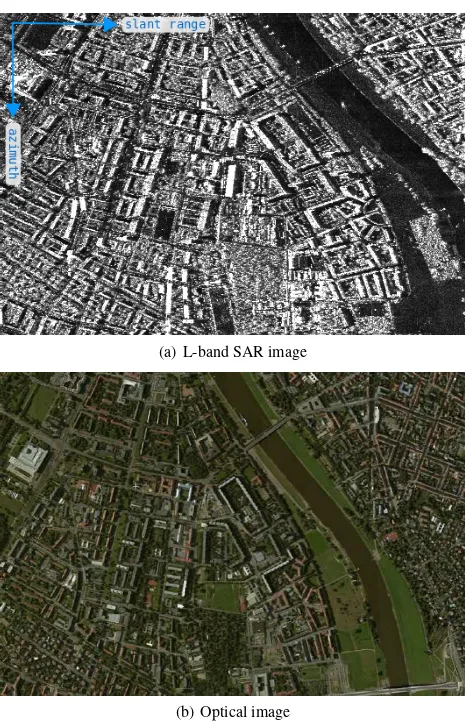
distortions in the SAR image, the crops cannot correspond per-fectly). Many vegetated areas can be seen on the corresponding optical image and the presence of trees between buildings can be noted. At this frequency band, tomographic imaging of buildings and ground through the canopy is possible due to the penetration of the microwaves. However, due to the low number of images, vegetation makes the tomographic imaging of such buildings dif-ficult. Moreover, geometric distortions due to the acquisition ge-ometry and the presence of speckle corrupting the intensity make a semantic interpretation challenging.
3. SAR TOMOGRAPHY 3.1 Acquisition Geometry and Layover
A SAR image is acquired thanks to a side-looking antenna lo-cated on a moving platform such as a plane or a satellite. The
(a) L-band SAR image
(b) Optical image
Figure 3: (a) SAR and (b) optical images of the selected area. Dimensions of the cropped SAR image are approximately of 700 pixels in azimuth and 1000 pixels in range. The optical image is from c"Microsoft Bing Maps, 2015
slant range
Figure 4: Illustration of tomographic SAR principle: due to the acquisition geometry of a SAR sensor, the backscattering of sev-eral targets may be superposed in the same pixel. This effect is called layover. Moreover, the altitudes are lost. To separate and localize these scatterers in the 3D space, SAR tomography com-bines several images acquired with slightly different incidence angles.
between the imaged objects, calledtargets, and the sent pulse. These echoes are then combined to form an image in a stage calledSAR focusing. Description of this procedure is beyond the scope of this paper and can be found in several publications, such as (Oliver and Quegan, 1998). SAR produces 2D complex im-ages where the pixel amplitude is due to the power backscattered to the sensor and the phase mainly depends on the distance to the object.
The image geometry is described by two coordinates, theazimuth
along the direction of flight and theslant rangewhich is the line-of-sight direction. Considering the platform at a particular az-imuth position, the received signal is time-gated in order to sep-arate the echoes of the different targets into pixels according to their corresponding time delays. Because the wave travels at the known speed of light, there is a straightforward relationship be-tween time delay and slant range coordinate in the SAR image.
Hence, objects are projected from the 3D space to the azimuth/ slant range coordinate system of the SAR. Therefore, the value of a pixel corresponds to the coherent sum of echoes from scatterers located within a given slant range interval, as shown in the ide-alized drawing of Figure 4. As depicted, if a non-flat structure is present, several targets with distinct 3D positions may have their contributions added into the same pixel. This effect is called lay-over.
In order to separate such contributions, SAR tomography uses several images of the same scene under slightly different view angles. The following section briefly explains how using an ap-propriate signal model and spectral methods allows to localize the 3D positions of targets.
Furthermore, multiple bounce scattering between ground, facade, tree trunks, etc may occur. These affect the phase and may cause wrongly located points in the tomographic point clouds. Double bounce scattering between ground and facade are typically char-acterized by bright lines in the image. Besides, due to the side looking geometry, building and ground parts may be located in the shadows of other structures, which are seen as dark areas in the image. Examples of such phenomena are illustrated in Figure 5.
double bounce
shadow
scattering
Figure 5: Example of other artifacts in SAR data. Multiple bounce and shadow occur (here we show the example of double bounce between a ground and a facade).
3.2 Signal Model
We consider K SAR images of the same scene acquired with slightly different angles. Assuming all the images have been co-registered to the geometry of one of them, calledmaster, we have a tomographic image stack with K-dimensional complex pixels. In SAR images with a resolution of the order of meters, a tar-get may contain many elementary scatterers due to the random-ness of media. This results in a phenomenon called speckle due to constructive and destructive interference between all elemen-tary scatterers, which can be modelled as a multiplicative noise (Goodman, 1984). Consequently, for the target vectork contain-ing the K complex values of a pixel in the tomographic stack we assume the following signal model (Lombardini et al., 2003):
k=
where$represents the Hadamard product,Nsis the number of targets,hiandτiare the height and reflectivity of targeti,xiis speckle vector of densityCN(0,Σxi),nis a Gaussian additive
noise vector of densityCN(0, σn2I)andais called thesteering
vector. Its elements areal = exp (−j4λπdl(hi))and contain phase information related to targetiand its distancedl(hi)to sensor l, whereλis the wavelength. The covarianceΣxi has
diagonal elements equal to 1and off-diagonal elements which depend on decorrelation effects.
3.3 Model Inversion
3.3.1 Sample Covariance Matrix First, standard steps such as de-ramping and phase calibration, to compensate possible er-rors on antenna location, are performed on the image stack. More details can be found in (Reigber and Moreira, 2000). From this signal, SAR tomography’s goal is to retrieve the vertical posi-tions of the targets. This problem can be recast as a Direction-Of-Arrival problem, solved by standard spectral estimation pro-cedures such as Beamforming, Capon and MUSIC (Stoica and Moses, 1997). These methods all require the estimation of the covariance matrixΣ =E(kkH).This matrix being unknown, it has to be estimated from the data by performing an average over
Li.i.d. samples (i.e.pixels):
C= 1
of a spatial resolution loss.
3.3.2 Tomographic Processing In this work we choose to use the MUSIC method assuming one scatterer per pixel (MUSIC-1). In (Sauer et al., 2011), it is shown to give the best results on this data for single polarization when compared to other approaches. The MUSIC method consists in maximizing the pseudo-power:
PM U SIC(h) =
1 a(h)HGGHa(
h) (3)
whereGis the matrix of covariance eigenvectors which span the noise subspace anda(h)is the steering vector computed at height
h. This pseudo-power is calledtomogramand itsNslocal max-ima give the wanted positions of the scatterers.
MUSIC-1 allows to extract for each pixel the height of the dom-inant scattering mechanism which leads to a 2D height map with the same dimensions as the image. Once the target heights are known, the points may be reprojected from the SAR geometry into the original ground geometry(x, y, z), leading to a 3D point cloud. In the following we refer to the termsheight mapwhen the points are in the SAR azimuth/slant range geometry andpoint cloudwhen the points have been re-projected in the original ge-ometry.
4. RADIOMETRY DRIVEN DETECTION OF BUILDINGS
4.1 Adaptive Covariance Estimation
Estimation of the covariance matrix by equation (2) leads to a trade-off between variance reduction and degradation of spatial resolution. If a high number of samples is used, edges between objects are blurred which may cause problems for the tomographic inversion and object detection. In order to mitigate this effect, we apply an adaptive procedure to improve the estimation of the covariance matrix without degrading edges. This filter was originally developed for polarimetric SAR data (D’Hondt et al., 2013b) and is based on the well-known bilateral filter. Applying this filtering for covariance estimation has two advantages. First, it reduces speckle on intensity which is useful for our radiome-try guided segmentation. Second, it improves the quality of the phase used in tomographic inversion, leading to a better quality height map.
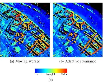
Figure 6 shows an example comparing the original intensity and the despeckled one obtained after applying the bilateral approach. Figure 7 shows how filtering the data prior to tomographic pro-cessing improves the quality of the 3D point cloud.
Note that a pre-estimation of the covariance matrix has first to be provided according to equation (2) on very small number of samples, which is a common practice in SAR image processing. In this work we perform a pre-summing of 3 along the azimuth coordinate.
4.2 Segmentation Driven Region Growing
Our building extraction method has been motivated by a few ob-servations:
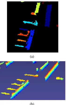
• Many buildings in the SAR image appear as bright struc-tures. This is due to the fact that the backscattering of large facades facing the sensor tend to dominate the overall re-sponse in layover areas. For these pixels, the estimated to-mographic heights are those of facades as MUSIC-1 esti-mates the height of the dominant scattering mechanism.
(a) Original (b) Filtered
Figure 6: Comparison of (a) original intensity image with speckle and (b) filtered image thanks to adaptive covariance estimation. The trace of the covariance matrix is displayed.
(a) Moving average (b) Adaptive covariance
min. height max.
(c)
Figure 7: Comparison of point clouds obtained with (a)5⇥5 boxcar and (b) adaptive covariance filtering. (c) Color coding of heights in this paper.
• Roofs of buildings which are not facing the sensor are well visible in the height maps. However, their reflectivity is low and they cannot easily be detected in the radiometric image.
• The assumption of planar patches to decompose building roofs into geometric primitives is made. Due to the large distance between the sensor and the imaged objects, the pro-jection of planar facades into the SAR geometry will also be well approximated by planes. Due to a smooth topography, the ground may also be approximated as locally planar.
• Most buildings have an elongated shape and rectilinear edges.
Example of facades and roofs seen in intensity image and tomo-graphic height map are shown in Figure 8.
Based on these observations, we have developed a building de-tection method exploiting the complementarity between the ra-diometric image and the purely 3D geometric information. Op-erations are carried on in the SAR geometry: incoherent tomo-graphic processing leads to dense height maps where the natural image connectivity of pixels can be used for segmentation.
In (D’Hondt et al., 2013a) a region growing procedure was intro-duced to extract the planar parts of buildings and ground. The idea is to collect pixels in a window and compute at each position plane parameters of typeh(i, j) = ai+bj+cwhereiandj
Figure 8: Comparison of roof and facades as they appear in (a) the intensity image and (b) the height maps obtained with tomogra-phy. Facade appear as bright structures in the radiometric image and heights ramps in the point cloud. Roofs have low amplitude in the image but are well visible in the height map.
the standard deviation of the points around the estimated plane. Then the patch with lowestσis retained to start growing a re-gion. Points connected to the patch are progressively added if their distance to the fitted plane is less than a threshold (which was set to3.5σin the cited work). Every time the area of the region doubles, the plane parameters andσare updated. When no pixels can be added to the region, its corresponding subset is removed from the data and the whole procedure is repeated until the dataset contains less points than a user defined number (this number corresponds to the expected proportion of outliers,i.e.
points that do not fit any plane).
In this work, we extend the previous approach by using the radio-metric image information to guide the region growing procedure. This allows a significant improvement in the quality of the ex-tracted regions. We first perform a simple pre-segmentation on the filtered image: the intensity image (the trace of the filtered covariance matrix) is computed and thresholded in order to sep-arate high reflectivity areas, which are likely to contain building facades, from low reflectivity ones. Then we apply independently the region growing procedure to these two pixel subsets.
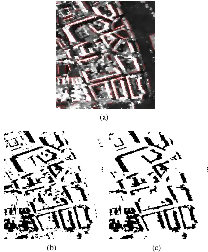
Prior to applying region growing to segmented high reflectivity regions, we eliminate regions that do not have rectilinear edges by applying the LSD (Line Segment Detector) to the intensity image (von Gioi et al., 2010). All connected components that do not intersect with a detected segment are discarded. The stages of our pre-segmentation procedure are illustrated in Figure 9.
Unfortunately, this procedure cannot be used for the subset of low reflectivity pixels since these structures do not have strong edges in the intensity image. Therefore, region shapes are examined in the classification step of the next paragraph to decide if they can be identified as building parts.
4.3 Identification of Building Parts
The region growing approach allows to identify planar primi-tives in the image. They potentially belong to roofs, facades and
(a)
(b) (c)
Figure 9: Illustration of image pre-segmentation: (a) detected lines (in red) superimposed with the radiometric image, (b) seg-mentation by thresholding intensity, (c) segseg-mentation with line segment information.
ground. Roofs can simply be distinguished from ground by their height. This is however not possible for facades. Therefore, we first identify facades by using the fact that they should be vertical when projected in the ground geometry. Hence, we compute the normal vector for each projected primitive and classify as facades the segments for which the absolute value of thezcomponent is lower than a threshold.
If a segment has been identified as a facade, it is added to the set of detected building parts. If not, we classify the segment as a roof if its mean height is higher than a threshold. For this data, the ground component is almost flat and roofs can be extracted this way. The approach could be extended in future works to terrains with stronger slope by identifying the ground components (as for example the components with the highest number of points) and computing the distance between a primitive and the plane corre-sponding to the closest ground component.
This classification step is applied to both high and low reflectivity primitives. The result of detection is finally the union of both classifications.
Additionally, because segments belonging to the low reflectivity subset have not been extracted with line segment information, we retain only regions with an elongated shape. For this, the eccentricity of the ellipse having the same second order moments as the region is computed and compared to a threshold.
5. EXPERIMENTS
(a) (b)
Figure 10: (a) Filtered covariance (intensity image) and (b) tomographic height map for the whole area of interest.
(a) (b)
Figure 11: Final segmentation results for both (a) high and (b) low reflectivity regions. Each building part is assigned a different color.
Extracting information of such data is challenging due to the low number of images and the moderate spatial resolution. The height map contains artifacts which may be due to the lack of precision in the flight path coordinates, decorrelation effects affecting the phase quality, occlusion of buildings by vegetation and multiple bounce scattering.
Figure 11 shows the segmentation labels obtained with our method. For the classification step, we used thresholds of0.3on the abso-lutezcomponent of the plane normals and20meters above the data’s minimum height for the roof detection. For low reflectiv-ity regions, we experimentally set the threshold on eccentricreflectiv-ity to 0.92. Unfortunately reference data was not available at the time of the experiment. It is however possible to visually assess our detection by comparing the results with the optical image, height map and SAR intensity image.
It is interesting to note that most segments extracted in the low reflectivity areas have an orientation that corresponds to buildings not facing the sensor. These segments mainly correspond to roofs that are not well visible in the intensity image.
It can be observed that the facades which have been correctly reconstructed by the tomographic processing are successfully ex-tracted by our method. Furthermore, the algorithm results in a significant improvement of the facade reconstruction thanks to the re-projection of points on their respective plane, as shown in Figure 12.
Figure 13 shows the outputs of the different stages of our method on a zoomed area: pre-segmentation, region growing over the
(a) (b)
(c) (d)
Figure 12: Examples of facade reconstructions. (a) and (c) show the original points, (b) and (d) show the reconstructed points after applying our extraction method. We have manually outlined the facades in the original point cloud for a better visualization.
(a) (b) (c) (d) (e)
Figure 13: Outputs of the different stages of our method on a cropped area. (a) Pre-segmentation used to guide region growing. (b) Region growing and (c) final segmentation over high reflectivity areas. (d) Region growing and (e) final segmentation over low reflectivity areas.
(a) (b)
Figure 14: Results of region growing where no pre-segmentation is used. Black rectangles show examples of bad segmentation that can be compared to results of Figures 13 and 15.
(a)
(b)
Figure 15: Segmentation result zoomed over the roof and facade areas of Figure 8. (a) Final segments (combined view of both high and low reflectivity areas). (b) 3D reconstructions of the corresponding building parts reprojected in the(x, y, z) geome-try.
ground and vegetated areas are discarded from the final segmen-tation. The region growing segmentation of the low reflectivity regions is of lower quality due to the absence of image edge in-formation to guide the procedure. However, several roofs that are not well visible in the radiometric image but appear in the tomo-graphic height map are successfully segmented by the method.
For comparison, Figure 14 shows the result of region growing without segmentation. This corresponds to the method
pre-sented in (D’Hondt et al., 2013a). In this case, several buildings are not well separated from the ground.
Finally, Figure 15 shows the result of the extraction method on the area presented in Figure 8 and the corresponding 3D point cloud of the reconstructed building parts. Here, the union of clas-sification over high and low reflectivity subsets is shown.
5.1 Limitations
Our method is suited for buildings that either have a large fa-cade facing the sensor or high roofs with a strongly anisotropic footprint. In the case of buildings with a non-rectilinear foot-print or roofs below the vegetation level, detection will fail due to the use of thresholds which are set globally. Our method also suffers from the data resolution and quality: pixels belonging to small buildings (e.g. houses) which are surrounded by vegeta-tion are likely to contain volume scattering from the canopy and multiple reflections due to tree trunks. With this low number of images, the tomographic resolution of many scatterers is not pos-sible. For this reason, some small buildings will not even appear in the height map.
The reconstruction of 3D planes also depends on the data qual-ity: some facades may appear slanted due to the low number of points and be possibly wrongly located due to multiple bounce scattering effects.
6. CONCLUSION
In this work we have proposed an approach to segment and re-construct building parts in tomographic SAR data which is suited for airborne data with moderate resolution. Unlike previous ap-proaches, we have considered points in the original image geom-etry. This allowed us to exploit edge information from the ra-diometric image in order to guide the segmentation of 3D planar regions. This edge information was incorporated through a pre-segmentation based on image reflectivity. The pre-segmentation was refined by the use of a line segment detection in the radiomet-ric image. In the height map, planar primitive identification was performed by a region growing approach exploiting the natural connectivity of pixels in the image geometry. The obtained prim-itives were then classified thanks to geometric tests to determine if they were building parts.
This approach was applied to experimental data and has allowed to extract elongated buildings. In the high reflectivity areas, most of the reconstructed structures are facades, whereas roofs are mostly present in the low reflectivity areas.
as regularization by Markov Random Fields. Detection of non-rectilinear and non-elongated buildings will also be addressed. This could be done by including more radiometric and geometric features in a machine learning based approach. Discrimination of vegetated areas could also be considered by incorporating texture information.
ACKNOWLEDGEMENTS
The authors would like to thank DLR for providing the E-SAR data. This work was supported by the German Science Founda-tion DFG, under project No. DH 75/2-1.
REFERENCES
Aguilera, E., Nannini, M. and Reigber, A., 2013. Wavelet-based compressed sensing for SAR tomography of forested areas. IEEE Trans on Geosc. and Remote Sensing PP(99), pp. 1–1.
Bamler, R. and Hartl, P., 1998. Synthetic aperture radar interfer-ometry. Inverse Problems 14(4), pp. R1.
D’Hondt, O., Guillaso, S. and Hellwich, O., 2013a. Geometric primitive extraction for 3D reconstruction of urban areas from to-mographic SAR data. In: Urban Remote Sensing Event (JURSE), 2013 Joint, pp. 206–209.
D’Hondt, O., Guillaso, S. and Hellwich, O., 2013b. Iterative bi-lateral filtering of polarimetric SAR data. Selected Topics in Ap-plied Earth Observations and Remote Sensing, IEEE Journal of 6(3), pp. 1628–1639.
Fornaro, G., Serafino, F. and Soldovieri, F., 2003. Three-dimensional focusing with multipass SAR data. IEEE Trans on Geosc. and Remote Sensing 41(3), pp. 507–517.
Gini, F., Lombardini, F. and Montanari, M., 2002. Layover so-lution in multibaseline SAR interferometry. Aerospace and Elec-tronic Systems, IEEE Transactions on 38(4), pp. 1344–1356.
Goodman, J. W., 1984. Statistical properties of laser speckle pat-terns. In: J. C. Dainty (ed.), Laser Speckle and Related Phenom-ena, second edn, Springer-Verlag, New York.
Guillaso, S. and Reigber, A., 2005. Polarimetric SAR tomogra-phy. In: POLINSAR’05, (Frascati, Italy).
Huang, Y., Ferro-Famil, L. and Reigber, A., 2012. Under-foliage object imaging using SAR tomography and polarimetric spectral estimators. Geoscience and Remote Sensing, IEEE Transactions on 50(6), pp. 2213–2225.
Lombardini, F. and Reigber, A., 2003. Adaptive spectral esti-mation for multibaseline SAR tomography with airborne l-band data. In: Geoscience and Remote Sensing Symposium, 2003. IGARSS ’03. Proceedings. 2003 IEEE International, Vol. 3, pp. 2014–2016.
Lombardini, F., Montanari, M. and Gini, F., 2003. Reflectiv-ity estimation for multibaseline interferometric radar imaging of layover extended sources. Signal Processing, IEEE Transactions on 51(6), pp. 1508–1519.
Oliver, C. J. and Quegan, S., 1998. Understanding Synthetic Aperture Radar Images. Artech House, Norwood, MA.
Reigber, A. and Moreira, A., 2000. First demonstration of air-borne SAR tomography using multibaseline L-band data. IEEE Trans on Geosc. and Remote Sensing 38(5), pp. 2142–2152.
Sauer, S., Ferro-Famil, L., Reigber, A. and Pottier, E., 2011. Three-dimensional imaging and scattering mechanism estimation over urban scenes using dual-baseline polarimetric InSAR obser-vations at L-band. Geoscience and Remote Sensing, IEEE Trans-actions on 49(11), pp. 4616–4629.
Shahzad, M. and Zhu, X. X., 2015. Robust reconstruction of building facades for large areas using spaceborne TomoSAR point clouds. Geoscience and Remote Sensing, IEEE Transac-tions on 53(2), pp. 752–769.
Stoica, P. and Moses, R., 1997. Introduction to Spectral Analysis. New Jersey: Prentice-Hall.
Tebaldini, S., 2010. Single and multipolarimetric SAR tomogra-phy of forested areas: A parametric approach. Geoscience and Remote Sensing, IEEE Transactions on 48(5), pp. 2375–2387.
von Gioi, R., Jakubowicz, J., Morel, J.-M. and Randall, G., 2010. LSD: A fast line segment detector with a false detection control. Pattern Analysis and Machine Intelligence, IEEE Transactions on 32(4), pp. 722–732.