A MINIMUM SPANNING TREE BASED METHOD FOR UAV IMAGE
SEGMENTATION
Ping WANG a, Zheng WEI a, *, Weihong CUI b, Zhiyong LIN b
a South China Sea Institute of Planning and Environment Research, SOA, Guangzhou, China b School of Remote Sensing and Information Engineering, Wuhan University, Wuhan 430079, China
Commission VII, WG VII/4
KEY WORDS: Statistical Learning, Minimum Spanning Tree (MST), Image Segmentation Rule
ABSTRACT:
This paper proposes a Minimum Span Tree (MST) based image segmentation method for UAV images in coastal area. An edge weight based optimal criterion (merging predicate) is defined, which based on statistical learning theory (SLT). And we used a scale control parameter to control the segmentation scale. Experiments based on the high resolution UAV images in coastal area show that the proposed merging predicate can keep the integrity of the objects and prevent results from over segmentation. The segmentation results proves its efficiency in segmenting the rich texture images with good boundary of objects.
* Corresponding author
1. INTRODUCTION
The ultimate purpose of image segmentation is to gain the maximum regional similarity within each segmented region and minimum regional similarity between segmented regions, which is a typical clustering and optimization problems. So optimization method can be used to solve this problem.
Image segmentation technology based on graph theory is a new research hotspot in the field of image segmentation in recent years (Santle and Govindan, 2012; Falcão et al., 1998). Graph theory, as a branch of mathematics, its research object is graph composed of a number of vertices and edges that is connected to the vertices (Mortensen and Barrett, 1998; Shi and Malik, 2000; Wei and Cheng, 1991; Xu et al., 2003). This graph can be used to describe the relationship between things, with vertices represent things and an edge between vertices corresponds to the relationship between the two things (Boykov and Jolly, 2001; Boykov and Kolmogorov,2004). Image segmentation algorithm based on graph theory method has been applied in medical image segmentation (Grady and Schwartz, 2006) and motion segmentation (Hickson et al., 2014), texture segmentation, target segmentation, and has obtained many achievements (Cour et al., 2005). This kind of method maps an image to a weighted graph, in which vertices represent the pixel or areas and every edge connects two pixels or area with a given weight reflecting the similarity between pixels or regions, then uses graph optimization theory to get the best image segmentation. Its essence is to switch image segmentation problem into optimization problem of graph theory so that image segmentation can be achieved based on the minimization of a cost function (Santle and Govindan, 2012) .
2. IMAGE SEGMENTATION BASED ON MST
Image segmentation method based on graph theory is mainly considering the influence from three aspects: a) cost function
reflecting the regional characteristics, b) optimal criterion for classifying of the graph, c) effective optimization algorithm (Felzenszwalb and Huttenlocher, 2004; Kropatsch et al., 2007).
2.1 The idea of MST based image segmentation
Minimum spanning tree (Xu and Uberbacher, 1997) problem in graph theory is the search for spanning tree with minimum sum of edge weights. Every tree is a connected graph. Therefore, image segmentation problem, which is looking for the connected regions with minimum differences, can be converted into minimum spanning tree problem. Image segmentation based on minimum spanning tree mainly uses two different strategies: a) top-down dividing and b) bottom-up merging. Top-down dividing strategy, based on a constructed image graph model, first uses the minimum spanning tree algorithm to get a minimum spanning tree that connects the whole image, and then divides the minimum spanning tree according to a certain principle. That process for image segmentation, especially the large image, will increase the amount of calculation. Therefore, this paper adopts a bottom-up merging (or regional growth) strategy to achieve image segmentation based on minimum spanning tree, which is called the minimum spanning tree method.
2.2 Image segmentation based on constructed MST
Image segmentation method, based on minimum spanning tree, is based on the constructed images model using the bottom-up merging strategy according to certain principle, in which the minimum spanning tree algorithm is used to construct minimum spanning tree that conforms to multiple criterion. Each minimum spanning tree represents a connected area, such as the traditional fixed threshold algorithm, single connection algorithm, fully connection algorithm, etc. The segmentation algorithm implementation process is described as follows:
(1) Construct the image graph model in which each pixel in image is vertex and an edge between two adjacent pixels (four-neighbourhood or eight-(four-neighbourhood) is linked together. The weight of edge is calculated according to the feature vector similarity of two vertices. As shown in Fig. 1-(b) and 1-(a), the image graph model are based on eight-neighbourhood, in which each black dots correspond to the image pixels and the edge weights value on the edge is the absolute pixel-value difference. (2) With the minimum spanning tree algorithm, such as Kruskal algorithm, the edges are sorted in order of non-decreasing order. Then the minimum spanning tree is constructed from the edge with the least weight value.
(3) If the current edge weights meet segmentation criteria (such as less than predefined global threshold value), add the edge into the spanning tree.
(4) Repeat steps (3) until the current edge weight does not meet the criteria (such as greater than the predefined global threshold value). Fig. 1-(c) and 1-(d) are the segmentation results with different global threshold. Among them, Fig. 1-(c) is the segmentation results of threshold 11, which contains two minimum spanning trees. Fig. 1-(d) is segmentation results of threshold 10, which contains three minimum spanning trees. That is to say that the image is segmented into three regions.
82 77 77 80 83
80 79 84 82 88
87 84 81 135 80
144 143 140 136 124
141 139 139 142 140
(a) pixel-value of image (b) Graph model of image
(c) Result with threshold 11 (d) Result with threshold 10 Fig.1 Image Segmentation based on minimum spanning tree of
graph model.
Results show that the result of simple threshold based image segmentation is sensitive to noise, especially when the threshold is set unreasonably. As shown in Fig 1-(d), due to the decrease of the threshold, more isolated points are produced. Therefore, it is needed to take measures to merge these isolated points to the most similar area. The most popular method is merge these isolated points to its adjacent area which the pixel with minimize differences belongs to in non-descending order. It can be found that 1) segmentation algorithm based on minimum spanning tree starts to merge from the pixel with smallest difference, which can avoid seed point selection problem and achieve the global optimal, but simple threshold criterion is sensitive to noise and easy to produce isolated point,
2) the process of merger is only influenced by the weights of edges, which has nothing to do with the original data. Certainly, it can be considered to take the original data and its neighbourhood relationship into consideration in the algorithm implementation and rules designing, but this will increase the computational complexity. Therefore, reasonable design of edge weight constructor and merger rules is very important.
3. MERGING RULES DESIGNING BASED ON SLT
Image segmentation process is a process of looking for homogeneous area and learning to judge. Image segmentation based on minimum spanning tree algorithm is a process of growing tree. It can be viewed as a small amount of similar samples looking for similar goals, and that is what the statistical learning theory is good at in the learning process. Therefore, the application of statistical learning theory in image segmentation criteria setting is feasible. This article regards image segmentation as a regression estimation problem, which converts the empirical risk minimization problem into a probability problem, and put forward a uniformly stable learning algorithm of the minimum spanning tree segmentation rules based on empirical risk minimization. As the rules only consider the features of the edge, it can avoid complex operations compared with traditional methods.
3.1
b
uniform stability algorithmTo clearly illustrate derivation process, several concepts and related theorems are given:
(1) Loss function. If given a x , the forecasted output value of
( )
f x , the actual value y *, then the loss is L f( ( ), *)x y , which is known as the loss function. This function is used to measure the predict performance of an algorithm. The commonly used loss function is square loss or L2 loss as shown below.
2
( , )
( ( ), *)
( ( )
*)
c f z
=
L f
x
y
=
f
x
-
y
(1)
(2) The generalization error. D f[S]I f[S]IS[fS]is the generalization
error, in which IS[fS] is the empirical risk and I f[ S] is the
expected risk. Our goal is to minimize I f[ S] but I f[S] is unmeasurable. We can define a error bound that the generalization error can reach and give it a limit. If IS[fS] is small, I f[ S] will be small too, which passes conformance ( D f[ ]S 0 , when l ¥). There are two methods to get generalization error bound: 1) to limit the size of the hypothesis space, 2) the use of the stability of the algorithm. This paper uses the second method. The basic idea is that when the training set has a slight disturbance, the function of limit algorithm has corresponding changes. This method does not care about "good performance" of all the functions, but only care about the probability that the generalization error bound of the algorithm is greater than a certain value, namely
(| [ ] [ ] | )
S S S S
P I f -I f >e <d
(2)
Given a training set S and a new training set Si z, in which point
i
is replaced by a new point z ÎZ.
We say algorithm has b uniform stability (b-stable
) if it satisfies:,
For each possible training set, replace arbitrary training point to other training point, if the loss at any point is no more than
b
, then the algorithm is stable. In fact, b =0 is that the best stability that we expect.Through McDiarmid inequality (McDiarmid, 1998), Bousquet and Elisseeff (2001,2002) have proved the probability of the generalization error bounds: stability, which means that the function is invariable no matter how the training set changes. So, for the error bound, using b =0 and probability 1-
, we will get the relationship between error bound, loss bound, number of samples and probability 1-
as follows.2 ln(2 / )
[ S] S[ S]
I f I f M
l (8) 3.2 Merging rules designing
This article views image segmentation as a predictive learning process to predict whether a pixel or areas should be merged into another area. So the aim is to find an algorithm fS to
produce an output yi for every input xi. Assuming that all
pixel values in a homogenous area are independent random variables belonging to a certain probability distribution P
.
1 1
(x ,y ) , , (xl,yl) come from P, xi is the observed pixel
grey value, yiis the corresponding true value, and y* is the
true grey value of the homogenous area. Therefore, every pixels merged into the same area satisfy fS( )xi xiyiyi*y*, which means for that area, IS[fS] =0 and the image segmentation based on minimum spanning tree is converted into a probability problem described in Eq. (8). Considering that the first step of Kruskal minimum spanning tree algorithm is to sort the edge weights in non-decrease order, that is to say that it begins to construct the MST from the edge with minimum weight between two most similar pixels.
Therefore, we see the grey levels of pixels as the real value of homogenous area. As the growth of the MST, edge weights joining into the MST are the increasing. The finally joined edge weight reflects the biggest loss of the observation area. So for
the MST, we have (n MST)e MST( )1, in which (n MST) is the number of points in MST, (e MST) is the number of edges in MST. According to the definition of loss function in Eq. (3), we can find that the edge weights function is the loss function and in the process of prediction, [ ]
S
which is used to judge whether this two region should be merged. '1
S I and '2
S
I are the empirical risk of region S1and S2,
which can be expressed as follows. 1
According to the empirical risk bound in Eq. (10), we can define the composed Merging Rule I:
1 2
It says that if the empirical risk of merging two areas connected by the same edge is no more than their corresponding generalization error bound, true is returned, otherwise false is returned.
From Eq. (11) and (12), we can see that the empirical risk is the average of edge weights in the region. That will increase the amount of calculation. So we can improve the Merging Rule I to get Merging Rule II.
The basic idea of Merging Rule II is to assume that every loss value is the worst, namely the maximum loss. It is corresponding to the last edge weight added to MST, which is exactly the edge we want to predict whether we should add or not. So, we have
weight added to MST at last. According to Eq. (4) and the explanation above, we will get the following probability expression.
With this, Merging Rule I can be improved to Merging Rule II
It can be seen from Eq. (16) that the Merging Rule II just need to compare the current edge weight with the generalization error bound of the two connected regions, which can reduce the amount of data storage and computation.
4. MERGING RULES ANALYSIS AND EXPERIMENT
4.1 Merging rules analysis
According to the derivation process of the two rules, we can find that:
1) They all use three parameters (ni,
,M) to control thethreshold, which are exactly the parameters to control the segmentation scale. ni is the number of pixels in region i and
is changing during the process of merging. The probability is a small value between 0 and 1, which doesn’t have big impact on the threshold. According to the theory of probability and the previous analysis, we usually set the value 0.1. M
i
s the upper bound of loss, it corresponds to the supremum of the edge weight. We can select the value of it according to the possible maximum edge weights. for grey image. Fig. 2 shows the changing curve of the threshold with the pixel number from 1 to 100 when d =0.1, and M is 30, 40, 50, 80, 100 and 120 respectively. It can be found that under the condition of two other parameters are fixed, the threshold value is larger when d is larger, which allows larger generalization error and large-scale segmentation result. For Rule I, Ii' is the average edge weights of MST. So to get be better segmentation result, M should be set as the average edge weights. For Rule II, M should be set as the maximum edge weight of the region we want.0 20 40 60 80 100
Fig.2 The relationship between the threshold and the area with different M.
2) When giving a low value to and M , the merging threshold decreases with the increase of region. This means that in the process of merging, large differences within the region were allowable with a small area, and as the area grows, smaller differences within the region were allowable, ensuring the consistency of the area, which makes the rule have better anti-noise performance, avoiding too small areas (over-segmentation). In Rule I, the edge weight average of MST was utilized to predict whether two areas were allowed to merge. It weakened the influence of the high edge weights. Therefore, it allows the large heterogeneity in the region. And the Rule II use the biggest edge weight to make prediction, so it can keep the regional internal consistency and boundary information. 3) Considering the amount of calculation, Rule I need to store each edge weight and calculate their sum and average. But Rule II just uses the current edge weight, which requires much less calculation and storage. In addition, in the process of constructing image model, it is easy to get maximum edge weights, i.e. the loss of the upper bound M . In this way, we can easily have a recommended value according to its value and internal difference allowed, so as to realize the division of different scale parameter.
To sum up, Rule II is better than Rule I in terms of accuracy and efficiency. This paper will further verify this judgement through experiment in Section 4.2.
4.2 Segmentation results and analysis
In this paper, we took remote sensing image data of Yangjiang in China (1:2000 scale DOM image generated by 800m altitude for 0.18 m resolution,which was acquired by UAV DM150 in November 28, 2014) as experimental objects, through two sets of segmentation experiments, the paper got comparative analysis of the minimum spanning trees based on two kinds of segmentation criteria ,which would also be compared with other segmentation methods.
In the first set of experiments, this paper compared the segmentation results of the two criteria presented by the paper itself.
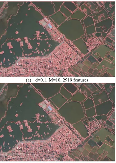
In case of d=0.1, M =1 0 and M = 1 5 , Figure 3 and 4 separately showed the results obtained from the Rule I and the Rule II (red curve for the regional boundary). As it can be seen from the figure, with the same parameters, Rule I segmented larger area and had greater differences within the region. On the one hand, this is because Rule I makes use of region weighted average, while Rule II the region maximum edge weights, which ensured the consistency of the region. On the other hand, for both two criteria, with the increase of the value of parameter M, the area of segmentation is also increasing. Therefore, different details of segmented regions would be got by choosing appropriate value of parameter M. Meanwhile, because of the same algorithm and the same idea of parameter control, segmentation results obtained by Rule I can also be achieved by Rule II. As it can be found from the figure, for both criteria, with the increase of segmentation scale parameter, internal details of the region were ignored, which guaranteed the features of integrity of the entire region segmentation. Namely, over-segmentation was avoided. Through the experiments,
better regional boundaries would be obtained by Rule II, without unnecessary detailed segmentation borders.
(a) d=0.1, M=10, 2919 features
(b) d=0.1, M=15, 1756 features Fig.3 Segmentation results by the Rule I.
(a)
d=0.1, M=10, 4786 features(b)
d=0.1, M=15, 3984 featuresFig. 4 Segmentation results by the Rule II.
(a) d=0.1,M=20, Rule II, 334 features
(b) Image part in the yellow line box of (a)
(c) k=255, 2803 features
(d) Image part in the yellow line box of (c) Fig. 5 Segmentation result comparison between the proposed
Rule II and the criterion proposed by Felzenszwalb.
In the second set of experiments, this paper compared the segmentation results of the Criteria 2 presented by the paper itself and the criteria proposed by Felzenszwalb and Huttenlocher (2004). Fig. 5-(a) showed the segmentation result obtained by Criteria 2 with M equalling 20, while Fig. 5-(c) showed the segmentation result achieved by Felzenszwalb Criteria with K equalling 255.As it can be seen from Fig. 5, the result obtained by Felzenszwalb Criteria exists many bilateral regions. As Fig. 5-(b) and 5-(d) in the yellow box partly displayed, these small bilateral regions were too trivial for region segmentation and object recognition, and they also easily led to small objects appearing in the interior of the whole region, such as the pond showed in the figure. When Felzenszwalb Criteria was made use of, many over-segmentation would appear, which is not conductive to the overall analysis. In addition, it can be seen from the figure, the method this paper presented can got a better ship boundary, while Felzenszwalb Criteria got many small objects around the ship, however, it can bitterly segment each small boats. Through a comparative analysis of the two sets of experiments above, it can be found that, the minimal spanning tree image segmentation criteria based on statistical learning theory presented by this paper can achieve the segmentation of different scales through scale parameter control, and has better anti- noise performance, better segmentation effect of texture regions and better regional boundaries.
Segmentation Rule proposed by this paper only considered the edge weight features. Because of the essential consistency of the minimum spanning tree based on bottom-up segmentation and region growing, seed point selection is a key step in region growing segmentation method, and the minimum spanning tree method start s growing from the most similar pixels, ensuring the global optimization, which provides a way to select the seed point of region growing method. Therefore, the combinative segmentation method based on the minimum spanning tree and the region growing method can be effective to improve the segmentation results. How to consider other factors besides edge weight features in the process of image segmentation into the segmentation criteria will be the next step of research.
5. CONCLUSIONS
Most object-oriented image segmentation method is essentially a process of regional growth. Seed point selection and the rationality of the design of segmentation criteria have important influence on the result of the division, which is the key and most difficult part of region growing segmentation method. Based on the optimization theory and algorithm of the minimum spanning tree in graph theory, this paper implements the regional growth type of object-oriented image segmentation, it gives priority to merge the most similar adjoining pixels, which can avoid the seed point selection problem of traditional region growth segmentation algorithm and at the same time take advantages of the minimum spanning tree algorithm and statistical learning theory to design the merging rules. This paper expounds the design rule of the segmentation of theoretical basis and the relationship between the segmentation parameters and the segmentation result is analysed. The experimental results, based on large scale unmanned aerial vehicle (UAV) digital orthogonal image in the coastal zone, show that the criterion has a good anti-noise performance and can get good texture region segmentation effect and obtain good area boundary.
At the same time, as the segmentation parameter selection is the important factors influencing the segmentation results, different terrain types need different segmentation parameters. Therefore, finding a set of segmentation parameter selection mechanism, to meet the needs of different images and terrain features, will be the further research direction of this paper.
ACKNOWLEDGEMENTS
This study is supported by the Public Science and Technology Research Funds Projects of Ocean (201305020-7), Open Research Fund Program of Shenzhen Key Laboratory of Spatial Smart Sensing and Services (Shenzhen University) (201302), the Director Fundation of South China Sea Branch of the State Oceanic Administration (1402), Natural Science Foundation of China (41101410), Natural Science Foundation of China (61527810) and Natural Science Foundation of Hubei (China) (2011CDB273).
REFERENCES
Bousquet, O. and A. Elisseeff. 2001. Algorithmic Stability and Generalization Performance. in Advances in Neural In-formation Processing Systems, 13. 2001.
Bousquet, O. and A. Elisseeff. 2002. Stability and generalization. Journal of Machine Learning Research, 2002, 2: p. 499-526.
Boykov, Y.Y. and M.-P. Jolly. 2001. Interactive Graph Cuts for Optimal Boundary & Region Segmentation of Objects in N-D Images. in International Conference on Computer Vision. July 2001: Vancouver, Canada,. p. 105-112.
Boykov, Y. and V. Kolmogorov. 2004. An Experimental Com-parison of Min-Cut/Max-Flow Algorithms for Energy Minimization in Vision. In IEEE Transactions on PAMI, 2004, 26(9): p. 1124-1137.
Cour, T., F. Benezit, and J. Shi. 2005. Spectral segmentation with multiscale graph decomposition, in IEEE Computer Vision and Pattern Recognition, 2005, 2: p. 1124-1131.
Falcão, A.X., J.K. Udupa, S. Samarasekera, S. Sharma, B.E. Hirsch, et al. 1998. User-Steered Image Segmentation Paradigms: Live Wire and Live Lane. Graphical Models and Image Processing, 1998, 60(4): p. 233-260.
Felzenszwalb, P.F. and D.P. Huttenlocher. 2004. Efficient Graph-Based Image Segmentation. International Journal of Computer Vision, 2004, 59(2): p. 167 – 181.
Grady, L. and E.L. Schwartz. 2006. Isoperimetric Graph Parti-tioning for Image Segmentation. IEEE Trans. Pattern Anal. Mach. Intell., 2006,28(3): p. 469-475.
Hickson S., Birchfield S., Essa I., and Christensen H. 2014. “Efficient Hierarchical Graph-Based Segmentation of RGBD Videos,” in Proceedings of IEEE Conference on Computer Vision and Pattern Recognition (CVPR), 2014.
Kropatsch, W.G., Y. Haxhimusa, and A. Ion. 2007. Multireso-lution Image Segmentations in Graph Pyramids. Studies in Computational Intelligence(SCI), 2007, 52: p. 3-41.
McDiarmid, C. in: M. Habib, C. McDiarmid, J. Ramirez-Alfonsin, et al. 1998. Concentration in Probabilistic Methods for Algorithmic Discrete Mathematics. 1998, Spring Verlag. p. 195-248.
Mortensen, E.N. and W.A. Barrett. 1998. Interactive Segmentation with Intelligent Scissors. Graphical Models and Image Processing, 1998. 60(5): p. 349-384.
Santle Camilus K., Govindan, V. K. 2012. A Review on Graph Based Segmentation, IJIGSP, 2012, 4(5): p.1-13.
Shi, J. and J. Malik. 2000. Normalized Cuts and Image Seg-mentation. IEEE Transactions on Pattern Analysis and Machine Intelligence (TPAMI), 2000, 22 (8): p. 888-905.
Wei, Y.C. and C.K. Cheng. 1991. Ratio cut partitioning for hierarchical designs. IEEE Transactions on Comput-er-Aided Design of Integrated Circuits and Systems, 1991, 10(7): p. 911-921.
Xu, N., R. Bansal, and N. Ahuja. 2003. Object segmentation using graph cuts based active contours. in IEEE Computer Vision and Pattern Recognition, 2003, 2: p. 46-53.
Xu, Y. and E.C. Uberbacher. e1997. 2D image segmentation using minimum spanning trees. Image and Vision Computing, 1997, 15(1): p. 47-57.