OVERLAND FLOW ANALYSIS USING TIME SERIES OF SUAS-DERIVED ELEVATION
MODELS
J. Jeziorskaa,b∗, H. Mitasovaa, A. Petrasovaa, V. Petrasa, D. Divakaranc, T. Zajkowskic
a
Department of Marine, Earth, and Atmospheric Sciences, North Carolina State University - (jajezior, hmitaso, akratoc, vpetras @ncsu.edu) bDepartment of Geoinformatics and Cartography, University of Wroclaw
c
NextGen Air Transportation (NGAT), Institute for Transportation Research and Education, North Carolina State University - (ddivaka2, tjzajkow @ncsu.edu)
KEY WORDS:UAS, UAV, sUAS, lidar, digital elevation model, overland flow modeling, path sampling
ABSTRACT:
With the advent of the innovative techniques for generating high temporal and spatial resolution terrain models from Unmanned Aerial Systems (UAS) imagery, it has become possible to precisely map overland flow patterns. Furthermore, the process has become more affordable and efficient through the coupling of small UAS (sUAS) that are easily deployed with Structure from Motion (SfM) algo-rithms that can efficiently derive 3D data from RGB imagery captured with consumer grade cameras. We propose applying the robust overland flow algorithm based on the path sampling technique for mapping flow paths in the arable land on a small test site in Raleigh, North Carolina. By comparing a time series of five flights in 2015 with the results of a simulation based on the most recent lidar derived DEM (2013), we show that the sUAS based data is suitable for overland flow predictions and has several advantages over the lidar data. The sUAS based data captures preferential flow along tillage and more accurately represents gullies. Furthermore the simulated water flow patterns over the sUAS based terrain models are consistent throughout the year. When terrain models are reconstructed only from sUAS captured RGB imagery, however, water flow modeling is only appropriate in areas with sparse or no vegetation cover.
1. INTRODUCTION
Mapping hydrological pathways by which water moves over and through the Earth surface is essential for explaining hydrologi-cal, geomorphologihydrologi-cal, ecological and geochemical phenomena (Hyv¨aluoma et al., 2013; Bevington et al., 2016). Precise and detailed representations of terrain are needed to accurately pre-dict overland flow. Therefore the acquisition of high resolution digital elevation data is necessary for accurately mapping over-land flow paths (Leit˜ao et al., 2015). Lidar – a technology that measures the distance to a target based upon the travel time of reflected light – is still at the forefront of high-resolution 3D data collection methods (Hodgetts, 2013). Novel methods for photo based 3D surface reconstruction, however, have opened a new pathway for developing solutions to affordably and efficiently generate very high resolution digital terrain models. Photogram-metric techniques have long been used to derive topographic data from analogue imagery such as stereo aerial photographs. Re-cent advances in computer vision computer algorithms coupled with the availability and affordability of digital cameras, how-ever, have lead to dramatic improvements in the collection and processing of terrain data using photogrammetry. The novel pho-togrammetric approach called Structure-from-Motion (SfM) en-ables fully automatic generation of high resolution digital terrain models using multi-view stereo techniques to derive 3D data from imagery taken with consumer grade cameras. This approach can be used to examine objects captured with terrestrial photographs as well as aerial imagery (Bemis et al., 2014). The rising number of applications and innovations is driven by the increasing acces-sibility of Unmanned Aerial Systems (UAS) technology. Until recently, most UAS applications were military. In the last decade, however, the emerging market for small (sUAS), light and easy to use systems led to UAS applications in industry, research and entertainment. Geoscientists have taken advantage of the integra-tion of sUAS and the SfM approach; numerous geoscience stud-ies have demonstrated the relevance, cost-effectiveness and
effi-∗Corresponding author
ciency of this approach. Procedures for obtaining imagery using unmanned platforms and processing acquired data in photogram-metric software no longer require expert knowledge and experi-ence. The high degree of automation in photogrammetric flight planning and execution and the availability of numerous software packages utilizing SfM algorithms make the extraction of three-dimensional coordinates from sufficiently overlapping photogra-phy possible (Tonkin et al., 2014) even without camera location and orientation data (Snavely et al., 2008; Westoby et al., 2012). It has been demonstrated that this approach produces terrain mod-els with resolution and data quality equivalent to or better than lidar (Carrivick et al., 2013; Fonstad et al., 2013). Legal pro-cedures, however, currently limit UAS data collection as regu-lations are still being adapted to this new, rapidly growing field (Summary of North Carolina Regulations concerning Unmanned Aircraft Systems, 2015).
It is clear that the photographs cannot replace lidar’s capability of obtaining the bare ground surface by filtering the vegetation cover. On the other hand the high cost of laser scanning surveys makes the acquisition of time series expensive. Cost may limit temporal resolution, a disadvantage when a study area undergoes frequent or sudden terrain changes. Arable land, for example, is subject to seasonal changes, crop rotation, and soil redistribution by intense tillage (Su et al., 2012; Ferreira et al., 2015). Further-more, arable land is susceptible to intensive erosion, which can modify its terrain and cause the formation of gullies (Ferreira et al., 2015).
significantly modify overland flow in cultivated areas, but also highlighted the DEM limitations in representing the flow pattern.
In this paper we propose a robust approach for analyzing micro-topography controls on surface water flow, drainage and ponding in agricultural landscape based on sUAS derived high-resolution elevation models. The objectives of this paper:
• to assess the suitability of digital surface models (DSMs) produced by sUAS photogrammetry for overland flow sim-ulation in the context of precision agriculture applications,
• to develop a workflow for overland flow pattern simulation using high spatial and temporal resolution DSMs derived from sUAS data, and
• to investigate the differences between flow patterns based on sUAS derived DSMs and lidar based DEMs.
The rest of the paper is organized as follows: first we introduce the data acquisition techniques and materials and we characterize the study area features. The next section is dedicated to method-ology of geoprocessing sUAS derived data and description of the algorithm used for overland flow modeling. After presenting re-sults of the research we summarize them in the last section that contains conclusions, discusses possible issues and suggests is-sues that are worth further investigation.
Figure 1: The targeted area, Lake Wheeler Road Field Laboratory of North Carolina State University, Raleigh, NC
2. STUDY AREA
The study area (Figure 1) is located within the jurisdiction of the City of Raleigh and Wake County, in the central region of North Carolina, USA at the Lake Wheeler Road Field Labora-tory of North Carolina State University (NCSU). Although lo-cated within the city limits, the farm is a part of delimited Special Area that has been identified by the local authorities as protec-tion area for maintaining water quality in the Swift Creek Wa-tershed (The 2030 Comprehensive Plan for the City of Raleigh, 2002). Current policy limits future development within the area. The majority of this protected area is now used for agricultural research.
Legal regulations regarding sUAS flights in North Carolina limit sUAS activity (Summary of North Carolina Regulations concern-ing Unmanned Aircraft Systems, 2015). The farm is located in one of the six areas in North Carolina for which NextGen Air
Transportation Group (NGAT) was granted the Certificates of Waiver or Authorization (COA). This authorization issued by the Air Traffic Organization to a public operator allows the holder specific legal UA activity within its borders.
The11.82ha area (35◦43′44′′N, 78◦41′54′′W) was selected based on the terrain features, changing land cover and presence of stable features such as roads. The elevation within the area varies from 105to120m a.s.l. Most of this area is arable land maintained by the Lake Wheeler Road Field Lab of North Carolina State Univer-sity. Soils within the area range from fine sandy loam to sandy loam and are classified are eroded due to intensive agricultural exploitation (City of Raleigh iMap portal, 2015).
3. DATA ACQUISITION
The time series of elevation data used for the analysis of sur-face water flow patterns was derived from imagery collected by repeated sUAS surveys of the study area over the time period of eight months. Airborne lidar data acquired for a 2013 Wake county survey were used to generate the reference DEM and DSM.
3.1 Unmanned Aerial System
The Unmanned Aerial System used in this study is UX5 pro-duced by Trimble. This system consists of a fixed wing aircraft and a designated tablet controller. The manufacturer provides a software for flight planning and control – Trimble Access Aerial Imaging application. This allows for an automated workflow and semi-autonomous flight. The airframe wingspan of 1 m and the weight of only 2.5 kg make the system suitable for a rapid deploy-ment, thus it can be used for monitoring post-storm landscape re-sponse. It cannot be used for observation during a storm, because the system is not able to operate in heavy rain and winds exceed-ing 65 km/h (Trimble, 2015). The onboard sensor is a consumer grade camera Sony NEX-5T capturing RGB imagery. In order to achieve the desired imagery resolution of about 3 cm, the flight ceiling during the executed flights was set to about100m (Ta-ble 1). The 14.8 V,6000mAh battery allows for50minute flight that can cover up to 19 km2
in one mission (Trimble, 2015). The flight mission can be prepared beforehand, with the full control of the desired quality of output products and the flight path.
3.2 Flight missions
The data were collected during five flights (Table 1) executed by NGAT in 2015 between the months of March and October to capture the changes in the fields during the growing season. There is a 225 days timespan between the first and last flight. All flights were executed after several days of significant rainfall except for the flight on September 21st flown after a dry period (Figure 2). In order to ensure the accuracy of the final results, multiple Ground Control Points (GCPs) were set in the field and the overlap of the photos was set to80 %in all the flights. De-pending on the visibility, 6 to 11 GCPs were identified during data processing.
3.3 Lidar data
Due to the rapid development of the Raleigh metropolitan area and the need of sustainable land management, high resolution el-evation data were recently acquired to support conservation plan-ning, design, research, floodplain mapping, and hydrologic mod-eling. This airborne lidar survey was the result of a project com-bining varied interests of Wake County, City of Raleigh and Town of Cary resulting in detailed multiple return and ground eleva-tion data covering approximately 2500 km2
Figure 2: Flight dates and daily precipitation between Mar 1, 2015 and Oct 31, 2015 for Lake Wheeler Rd. Field Lab Station
date resolution GCPs error density altitude
[cm/px] [px] [pts/m2] [m]
Mar 18 3.11 6 0.047 64.73 88
Jun 20 3.31 11 0.080 63.75 100
Sep 21 3.12 6 0.091 63.88 100
Oct 06 3.12 9 0.125 63.80 100
Oct 29 3.18 9 0.135 61.63 100
Table 1: Properties of sUAS surveys performed in the year 2015: date, ground resolution of the photos, number of GCPs, GCPs error, point densities and flight altitude. All surveys were flown
after significant rainfall period, except for Sep 21.
completed in February 2013 using ALS70 HP at2750m a.g.l., 40◦field of view,11 %minimum sidelap,0.82m average point spacing. All deliverables met or exceeded standards for both ver-tical and horizontal accuracy of95 %confidence for 0.623 m (2 ft) contours, according to NDEP Guidelines for Digital Elevation Data (NDEP, 2004). The classified point cloud from this survey was used to generate reference DEM and DSM for the study area.
4. METHODS
To perform the high resolution surface flow analysis a series of 0.3 m resolution DSMs was generated from the lidar and sUAS derived point clouds. The DSMs were evaluated for accuracy and geometric distortions using the GCPs and lidar based DSM. Overland flow was then simulated for a given design storm using path sampling method for solution of bivariate shallow water flow equations. The processing of sUAS imagery was performed in PhotoScan Professional by Agisoft (Agisoft, 2013), computation of DSMs and flow analysis was carried out using GRASS GIS (Neteler et al., 2012).
4.1 Photogrammetric UAS data processing
The images acquired by UAS were processed using structure from motion (SfM) to derive orthophotography and 3D point clouds. This technique – designed for extraction of 3D coordinates from sufficiently overlapping photography adjusted to the needs of UAS data – has been implemented in several photogrammetric soft-ware packages. After evaluation of several proprietary and open-source solutions, the software PhotoScan Professional by Agisoft was chosen for UAS data processing in this study. This system provides a semi-automatic, intuitive workflow and supports cus-tom settings in each step of geoprocessing. It is widely used in the research, i.e. (Gonc¸alves and Henriques, 2015; Leon et al., 2015; Javernick et al., 2014; Uysal et al., 2015), because of its solid performance and relatively efficient processing.
Agisoft PhotoScan is a proprietary package, thus the algorithms utilized during geoprocessing are not fully documented (Gonc¸alves and Henriques, 2015). The final products of the standard work-flow, described by manufacturer (Agisoft, 2013) are an orthomo-saic and a Digital Surface Model (DSM).
After the visual inspection of the photographs, the relevant im-agery is loaded to the program and the preliminary adjustment is executed using the camera orientation log. Image feature points (geometrical similarities) and their movement throughout the se-quence of multiple images is monitored and based on this infor-mation feature points are rendered as a 3D sparse point cloud. This procedure can be executed also without the information about the external orientation of a camera that is included in the flight log. The correct values of localization (coordinates, altitude) and orientation (pitch, yaw, roll) parameters of a sensor at the moment of photo capture are determined in the aerial triangula-tion process, but the processing is faster if approximate values for these parameters are known. This procedure is coupled with camera self-calibration, which resolves the issue of using a non-photogrammetric camera, although the inaccuracy of these esti-mates together with the algorithms used by the software cause the deformation known as a doming error (James and Robson, 2014). The issue can be resolved by performing optimization based on ground control data. The GCPs are identified on each photo, where the marker is visible and the optimization is carried out based on the known, pre-measured and accurate positions of the ground points.
The construction of dense point cloud is performed by calculating depth maps for every image. PhotoScan determines the quality of the generated point cloud, but the more accurate the camera position estimates are, the more time and memory intensive the process will be. For our study the medium quality setting was chosen based on the memory required for the number of photos included in the processing. Efficient processing was possible only in a special height-field mode available in PhotoScan, which is highly optimized for aerial imagery (Agisoft, 2013).
Further steps recommended by the manufacturer – meshing and texture generation – are necessary for generating DSMs and or-thophotos in the software. We, however, decided to export the raw, georeferenced point cloud from PhotoScan and generate all DSMs with the same technique as the lidar based point cloud in order to compare the results of overland flow simulations based on data acquired by lidar and UAS. The orthophoto, produced with default values in PhotoScan was used for the validation pur-poses.
4.2 Classification and interpolation of point clouds
In order to model and compare water flow on raster DSMs from two completely different sources of elevation data – lidar and sUAS SfM – we derived all the DSMs from raw points clouds using the same technique, giving us control over the desired res-olution and level of detail captured in the resulting DSMs. The process consists of removing tree crowns from the point clouds and interpolating the DSMs using regularized spline with tension (Mitasova et al., 2005).
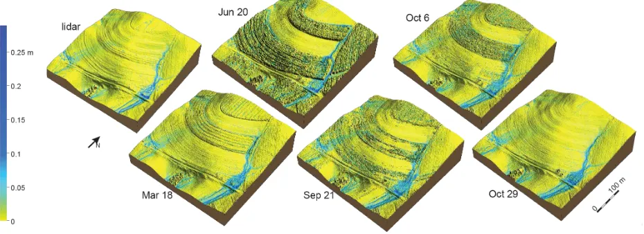
Figure 3: Overland flow pattern simulated for the lidar based DEM and DSMs based on the sUAS derived data in 5 flights in 2015
.
Figure 4: Differences in elevation between the lidar and sUAS based terrain models from the March flight. Figure A shows in blue areas where sUAS based DSM is higher than lidar. In B we show the difference after applying the shift correction and the inset shows
the differences higher than 1 cm of overland flow depth simulated on these two DSMs.
and Hudak, 2007) implemented in v.lidar.mcc tool (Blumentrath, 2014) available in GRASS GIS. Although originally designed for lidar data, this method is suitable for sUAS based point clouds be-cause it doesn’t require point return type. We successfully identi-fied and filtered high vegetation from the point clouds, however, not surprisingly, it was not possible to distinguish low vegetation such as crops and bushes due to their high density and small num-ber of ground points. Lidar data were already classified by the vendor and therefore we used bare ground class for further pro-cessing. We derived all sUAS based DSMs and lidar bare earth surface at 0.3 m resolution. Since we want to compare the flow patterns at the same resolution, we chose this resolution as it is still suitable for sparser lidar data and at the same time we do not loose too much detail of the dense sUAS data. The lidar data were interpolated using regularized spline with tension implemented in GRASS GIS as v.surf.rst module (Mitasova et al., 2005). We used a relatively low tension value of 20 and with smoothing value set to 1 to suppress the pattern of the scan lines while preserving the tillage surface geometry. The sUAS data were then processed in the same way.
To assess the possible influence of spatial distortion of the SfM reconstruction on water flow patterns, we analyzed the differ-ences between sUAS DSMs and lidar data. For each DSM, we computed a corrected DSM by extracting a trend surface from the difference to lidar and subtracted it from the original DSM. We derived the trend surface by computing median of the dif-ference using moving window with large size (100 m). Prior to
that we removed areas of difference higher than 10 cm to not in-fluence the trend by vegetation. The original and the corrected DSM were then compared in regard to water flow patterns, to see whether DSMs’ distortions of such magnitude matter for water flow pattern.
4.3 Overland flow simulation
Flow modeling at sub-meter resolutions is challenging due to high complexity of the terrain surface, including extensive nested real depressions. Surface flow modeling methods that rely on a depressionless DEM require substantial modification of this type of high resolution DEM, limiting the capability to capture the impacts of microtopography on the flow pattern or on ponding in the depressions. The path sampling technique, also referred to as Green’s function Monte Carlo, has been proposed as a robust, mesh-free alternative for solving the shallow water flow conti-nuity equation on complex surfaces (Mitasova et al., 2004). The technique is based on duality between the particle and field repre-sentation: in this concept, the density of particles in space defines a field and vice versa, a continuous field is represented by parti-cles (path samples) with corresponding spatial distribution. Us-ing this duality, processes can be modeled as evolution of fields or evolution of spatially distributed particles.
more details in Mitasova et al. (2004)):
−2ε∇2h5/3
+∇ ·(hv) =ie (1)
wherehis the depth of overland flow [m],vis flow velocity
vec-torv= (vx, vy)[m/s],ieis rainfall excess (rainfall−infiltration
−vegetation intercept) [m/s], andε is a spatially variable dif-fusion coefficient. The difdif-fusion term, which depends onh5/3
instead ofh, makes the Equation (1) linear in the functionh5/3
which enables us to solve it by the Green’s function path sam-pling method. The solution is then described as a function with statistical error proportional to1/√M whereM is the number of walkers. Incorporation of the spatially variable diffusion term
ε supports approximate simulation of water depth evolution in locations with flat topography and depressions. By defining the diffusion term as a function of water depth and the velocity of flow as a function of an approximate water flow momentum, wa-ter fills the depressions and flows out in the prevailing flow direc-tion. The method was implemented in GRASS GIS in the module r.sim.water.
We used path sampling to simulate shallow overland water flow and ponding in depressions for a design storm, assuming uniform rainfall excess rate of30mm/hr and a uniform surface roughness coefficient 0.15. For each DSM in the time series we ran the simulation at0.3m resolution for40minutes until steady state was reached in most of the modeled area.
Figure 5: Areas of a special importance, enlarged on figures 6, 7, 8, and 9
5. RESULTS AND DISCUSSION
In this section we present the results of the overland flow sim-ulation based on sUAS and lidar derived data. We focus on the differences in the generated terrain models that are the source of the discrepancies between final simulations. We analyze the generated overland flow patterns and validate them based on the orthophotos depicting actual conditions of terrain during sUAS data acquisition.
5.1 Assessment of DSM time series accuracy and spatial pat-tern of distortions
The assessment of the 2013 lidar DEM accuracy based on the 12 available GCPs (installed in 2015) confirmed its high accuracy with mean difference of5cm and RMSE of8.7cm.
Figure 6: Enlarged area A from Figure 5, with the visible gully
The mean differences between DSMs derived from aUAS surveys ranged from −0.1cm in March to 36.6cm in June (Table 2) and RMSE ranges from1.3cm in March to39.2cm in June and the spatial distribution of differences varies between the flights. The differences between the example SUAS derived DSM from March and lidar based DEM is shown in Figure 4.
Figure 7: The puddle on the service road (enlarged area C from Figure 5) captured on the orthophoto from Mar 18 (A and B), Jun 20 (C), Oct 06 (D) and Oct 29 (E) with displayed results of
overland flow simulations on lidar based DEM (A) and DSMs based on sUAS data collected Mar 18 (B), Jun 20 (C), Oct 06
(D) and Oct 29 (E)
Section 4.2. The comparison of the result on March DSM shows that spatial distortions of such magnitude can slightly alter the distribution of water on the landscape. They do not, however, significantly affect the patterns of water flow. Based on these finding we show here the water flow simulation results computed on the original DSMs.
The DSMs were generated using the same parameters (see the methods) but the accuracy of the results varied (Table 1) based on the flight conditions and availability of GCPs. The second flight in October produced relatively low quality images due to windy conditions and trouble placing GCPs.
Comparison of DSMs with lidar based DEM revealed spatially variable pattern of geometric distortions (Figure 4). As predicted,
date RMSE mean
Mar 18 11.5 -0.1
Jun 20 62.6 -36.7
Sep 21 20.0 8.3
Oct 06 15.7 1.6
Oct 29 19.3 13.9
Table 2: Comparison of lidar based DSM and sUAS derived DSMs, RMSE – root-mean-square error [cm], mean – mean
difference between lidar DSM and sUAS DSM [cm],
Figure 8: Enlarged area B from Figure 5, with the visible gully
the presence of the mature corn plants made it impossible to cap-ture the bare ground with the sUAS camera and resulted in cre-ating an artificial surface at the height of the plants. The DSM based on the June data shows the greatest differences compared to the lidar DEM with the mean of absolute values of differences as high as (see Figure 4 and Table 1)−36.7cm. This will signif-icantly influence the simulated flow pattern described below. The other area with substantial differences is located at the foothill and therefore does not influence the flow pattern.
5.2 Evolution of the overland flow pattern
The results of the overland flow simulation show a persistent, rel-atively stable flow pattern in spite of changes in the field due to tillage, crop growth and harvest (Figure 3). Small gullies were observed in the fields (Figure 5 A, B) and water ponded in de-pressions on the service roads (Figure 5 C, D). sUAS data cap-tured the redirection of flow and accumulation of water caused by tillage with greater detail than the lidar data. It is clearly vis-ible in the areas not covered by vegetation. The growing crops significantly disturb the flow pattern, creating an artificial pond-ing effect caused by representpond-ing the height of the corn as the elevation surface.
Figure 9: The puddle along the service road (enlarged area D from Figure 5) captured on the orthophoto from Jun 20 (A and B), Oct 06 (C) and Oct 29 (D) with displayed results of overland flow simulations based on lidar based DSM (A) and sUAS data collected Jun
20 (B), Oct 06 (C) and Oct 29 (D).
however during September and October the gully is disrupted by the presence of vegetation resulting in less clear but still recog-nizable shape. There are two explanations for the absence of the gully in the lidar data. Since the lidar survey was conducted two years before capturing the sUAS imagery, the gully could have developed after the lidar data collection. It is also possible that due to the lower detail of lidar based data the micro changes in the terrain are not well represented (similar to the tillage pattern) and the simulation reflects this simplified micro relief. While li-dar data can be helpful for identifying areas vulnerable to erosion, sUAS based data is needed to identify and monitor gully forma-tion.
5.3 Prediction and validation of water ponding on service roads
As there has not been any direct monitoring of runoff during storms, we validated the prediction of water flow patterns by comparing ponding on service roads predicted in the simulation with the actual situation in the field known from the orthophotos generated as part of the SfM reconstruction. In the orthopho-tos from June and both October missions several puddles appear along the unpaved road in the southern part of the targeted area (Figure 5 C, D). Despite the fact that puddles of turbid water are interpreted as ground surface by the SfM algorithm and thus we cannot accurately represent the local depressions, we hypothe-sized that the sUAS derived data still provide more accurate rep-resentation of the overland flow pattern than lidar data. Simula-tion based on the lidar DEM1(Figure 9, A) does not predict the water accumulation along the road (Figure 5 D), while the shape of the puddle aligns with the sUAS based simulations in all cases (Figure 9, B, C, D). This is also confirmed for the smaller pud-dle (Figure 5 C), where the water is visible additionally after the March rainfall (Figure 7). Our results show that sUAS derived data allow for accurate spatial prediction of surface water on ser-vice roads which provides valuable information for road mainte-nance and assessment of accessibility after storms. It can improve delineation of the potentially inundated areas and thus enables
1
There was no orthophoto available for the time of lidar data survey.
landowners to adjust water management practices and prevention procedures.
6. CONCLUSIONS
Agricultural areas are characterized by frequent changes in mi-crotopography that influence the surface water flow. It is there-fore crucial to obtain the most recent and detailed representation of terrain surface for overland flow modeling. This study investi-gated the possibility of using high spatial and temporal resolution data acquired by small Unmanned Aerial System for mapping flow paths. The results have been compared with the simulations based on the lidar derived DEM and the following conclusions have been drawn:
• sUAS derived data can improve the quality of the flow pat-tern modeling due to the increased spatial and temporal res-olution. It can capture preferential flow along tillage that is represented by capturing the changing microtopography.
• Overland water flow modeling based on data from airborne lidar surveys is suitable for identifying potentially vulnera-ble areas. sUAS based data, however, is needed to actually identify and monitor gully formation.
• Due to the high resolution of obtained data, vegetation sig-nificantly disrupts the flow pattern. Therefore densely vege-tated areas are not suitable for water flow modeling.
Future work will concentrate on eliminating the artificial ponding effect by replacing parts of the sUAS derived data covered with dense vegetation with the bare earth lidar point cloud. These sim-ulations extended by new data from future flight will be used for designing a validation experiment.
References
Agisoft, 2013. Agisoft PhotoScan User Manual: Professional Edition. Version 1.0.0 edn.
Bemis, S. P., Micklethwaite, S., Turner, D., James, M. R., Ak-ciz, S., Thiele, S. T. and Bangash, H. A., 2014. Ground-based and uav-Ground-based photogrammetry: A multi-scale, high-resolution mapping tool for structural geology and paleoseis-mology. Journal of Structural Geology69, Part A, pp. 163 – 178.
Bevington, J., Piragnolo, D., Teatini, P., Vellidis, G. and Morari, F., 2016. On the spatial variability of soil hydraulic properties in a holocene coastal farmland.Geoderma262, pp. 294 – 305.
Blumentrath, S., 2014. v.lidar.mcc GRASS GIS module.
Brasington, J., Vericat, D. and Rychkov, I., 2012. Modeling river bed morphology, roughness, and surface sedimentology using high resolution terrestrial laser scanning.Water Resources Re-search48(11), pp. n/a–n/a. W11519.
Carrivick, J. L., Smith, M. W., Quincey, D. J. and Carver, S. J., 2013. Developments in budget remote sensing for the geo-sciences.Geology Today29(4), pp. 138–143.
City of Raleigh iMap portal, 2015. Environmental layers group; Soils layer.
Evans, J. S. and Hudak, A. T., 2007. A multiscale curvature al-gorithm for classifying discrete return LiDAR in forested en-vironments. IEEE Transactions on Geoscience and Remote Sensing45(4), pp. 1029–1038.
Ferreira, V., Panagopoulos, T., Cakula, A., Andrade, R. and Arvela, A., 2015. Predicting soil erosion after land use changes for irrigating agriculture in a large reservoir of southern portu-gal. Agriculture and Agricultural Science Procedia4, pp. 40 – 49. Efficient irrigation management and its effects in urban and rural landscapes.
Fewtrell, T. J., Duncan, A., Sampson, C. C., Neal, J. C. and Bates, P. D., 2011. Benchmarking urban flood models of vary-ing complexity and scale usvary-ing high resolution terrestrial lidar data.Physics and Chemistry of the Earth, Parts A/B/C36(78), pp. 281 – 291. Recent Advances in Mapping and Modelling Flood Processes in Lowland Areas.
Fonstad, M. A., Dietrich, J. T., Courville, B. C., Jensen, J. L. and Carbonneau, P. E., 2013. Topographic structure from motion: a new development in photogrammetric measurement. Earth Surface Processes and Landforms38(4), pp. 421–430.
Gonc¸alves, J. and Henriques, R., 2015. UAV photogrammetry for topographic monitoring of coastal areas.ISPRS Journal of Photogrammetry and Remote Sensing104, pp. 101 – 111.
Hodgetts, D., 2013. Laser scanning and digital outcrop geology in the petroleum industry: A review. Marine and Petroleum Geology46, pp. 335 – 354.
Hyv¨aluoma, J., Lilja, H. and Turtola, E., 2013. An anisotropic flow-routing algorithm for digital elevation models. Comput-ers and Geosciences60, pp. 81 – 87.
James, M. R. and Robson, S., 2014. Mitigating systematic error in topographic models derived from UAV and ground-based image networks. Earth Surface Processes and Landforms 39(10), pp. 1413–1420.
Javernick, L., Brasington, J. and Caruso, B., 2014. Modeling the topography of shallow braided rivers using structure-from-motion photogrammetry.Geomorphology213, pp. 166 – 182.
Leit˜ao, J. P., Moy de Vitry, M., Scheidegger, A. and Rieckermann, J., 2015. Assessing the quality of digital elevation models ob-tained from mini-unmanned aerial vehicles for overland flow modelling in urban areas. Hydrology and Earth System Sci-ences Discussions12(6), pp. 5629–5670.
Leon, J., Roelfsema, C. M., Saunders, M. I. and Phinn, S. R., 2015. Measuring coral reef terrain roughness using Structure-from-Motion close-range photogrammetry. Geomorphology 242, pp. 21 – 28. Geomorphology in the Geocomputing Land-scape: GIS, DEMs, Spatial Analysis and statistics.
Mitasova, H., Mitas, L. and Harmon, R., 2005. Simultaneous spline approximation and topographic analysis for lidar eleva-tion data in open-source GIS. IEEE Geoscience and Remote Sensing Letters2, pp. 375–379.
Mitasova, H., Thaxton, C., Hofierka, J., McLaughlin, R., Moore, A. and Mitas, L., 2004. Path sampling method for modeling overland water flow, sediment transport, and short term terrain evolution in Open Source GIS.Developments in Water Science 55, pp. 1479–1490.
NDEP, 2004. Guidelines for digital elevation data.
Neteler, M., Bowman, M., Landa, M. and Metz, M., 2012. GRASS GIS: a multi-purpose Open Source GIS. Environmen-tal Modelling & Software31, pp. 124130.
Snavely, N., Seitz, S. and Szeliski, R., 2008. Modeling the world from internet photo collections.International Journal of Com-puter Vision80(2), pp. 189–210.
Su, Z., Zhang, J., Qin, F. and Nie, X., 2012. Landform change due to soil redistribution by intense tillage based on high-resolution DEMs.Geomorphology175176, pp. 190 – 198.
Summary of North Carolina Regulations concerning Unmanned Aircraft Systems, 2015.
Tonkin, T., Midgley, N., Graham, D. and Labadz, J., 2014. The potential of small unmanned aircraft systems and structure-from-motion for topographic surveys: A test of emerging inte-grated approaches at cwm idwal, north wales.Geomorphology 226, pp. 35 – 43.
Trimble, 2015. Trimble UX5 Unmanned Aircraft System. Datasheet.
Uysal, M., Toprak, A. and Polat, N., 2015. DEM generation with UAV photogrammetry and accuracy analysis in sahitler hill. Measurement73, pp. 539 – 543.
Westoby, M., Brasington, J., Glasser, N., Hambrey, M. and Reynolds, J., 2012. Structure-from-Motion photogrammetry: A low-cost, effective tool for geoscience applications. Geo-morphology179, pp. 300 – 314.

![Table 2: Comparison of lidar based DSM and sUAS derivedDSMs, RMSE – root-mean-square error [cm], mean – meandifference between lidar DSM and sUAS DSM [cm],](https://thumb-ap.123doks.com/thumbv2/123dok/3217001.1394735/6.595.115.230.657.737/table-comparison-based-deriveddsms-rmse-square-error-meandifference.webp)
