Finite volume modelling of free surface draining vortices
F. Trivellatoa;∗, E. Bertolazzia, B. Firmaniba
Dipartimento di Ingegneria Civile ed Ambientale, Universita degli Studi di Trento, via Mesiano 77, I-38050 Trento, Italy
bDipartimento di Ingegneria Meccanica e Strutturale, Universita degli Studi di Trento, via Mesiano 77, I-38050 Trento, Italy
Received 4 November 1998
Abstract
The phenomenon of the free-surface vortex forming over a draining intake is well known, together with its detrimental eects. While analytical solutions have been helpful in clarifying some features of the phenomenon, no extensions have been readily provided in solving instances of practical importance. Therefore, ecient anti-vortex devices have been traditionally conceived by means of physical model studies. However, a numerical simulation of the whole ow eld would be nowadays desirable. The proposed numerical solution of the ow eld is based on an axial-symmetric nite volume model, which solves the incompressible Navier–Stokes equations on irregular geometries. Boundary conditions include both the Dirichlet and the Neumann type. The mesh is staggered. The numerical scheme is a semi-implicit one, where the terms controlling the diusion and those controlling the pressure eld are discretized implicitly, while the convective terms are approximated via an Euler–Lagrange approach. The discrete version of the continuity equation becomes, by a substitution, a system having the pressure values as the only unknowns. The solution proceeds via an iterative scheme, which solves a symmetric and semi-positive-denite system for the pressure, by a standard pre-conditioned conjugate gradient method. The discrete velocity eld at each iteration can then be explicitly obtained. The numerical solution has been veried by the laboratory experimental data obtained by Daggett and Keulegan (1974). This comparison demonstrated that the proposed numerical model is capable of predicting the whole steady ow eld. Of special value is the comparison with the radial velocity distribution, which has a typicaljet-likeprole along the vertical direction. According to the most recent experimental evidence, it seems that the very onset of the vortex can be traced to this special feature of the radial velocity prole. c1999 Elsevier Science B.V. All rights reserved.
Keywords:Incompressible Navier–Stokes; Finite volume
1. Introduction
Intake draining vortices are free surface vortices forming over a hole discharging from a reservoir (Fig. 1). They occur typically whenever the submergence (or head of water) is less than a critical value.
∗Corresponding author.
Fig. 1. Sketch of the problem and notation.
The knowledge of the critical submergence is of the outmost relevance to the hydraulic engineer, in order to avoid the negative eects due to the vortex formation (such as, for instance, reduction of the discharge coecient, air entrainment, ingestion of oating debris and, at times, elimination of a serious safety hazard).
Several approaches have been presented in the literature to deal with the problem: that is, to determine whether or not an intake is prone to vortex formation. Basically, these approaches can be labeled as analytical models, physical models and, recently, numerical models.
Many analytical approaches have been presented in the literature in order to attain a theoretical view of the far-eld velocity (see, for instance, [7, 8, 13, 14]); still, the ow representation has deed so far any comprehensive analytical analysis. In fact, no mathematical model capable of representing the structure of the ow eld in the free surface vortex has obtained so far general consensus, so that a certain degree of confusion arises when reviewing the literature, which covers from rened theories (yet unpractical or without a sounding physical basis), to a model as simple as the well-known Rankine vortex.
Besides of being somewhat laborious and unpractical, the known analytical theories apply only to a limited range of vortices and have weak experimental validation.
Anwar [1], proposed an ingenious solution based on the method of separation of variables, which depended however on a couple of oversimplifying assumptions.
The structure of the ow pattern in the far-eld domain cannot be tackled by similarity analysis: the attempts conducted so far have not lead to any useful results and the problem does not seem to admit a similarity variable, either of the form =ra=zb (a and b any constant) or, more in general,
A simple, yet eective method for the representation of the far-eld ow, was devised by Cola and Trivellato [5]. The method is based on potential ow theory by adopting a suitable arrangement of image sinks. The comparison with the Daggett and Keulegan [6] experimental data was fairly accurate up to a distance as close to the intake as r≃1:7R0; and demonstrated that the bottom
boundary layer can be safely neglected in calculations.
Analytical models (a review of which can be found in [5, 21, 22]), have all been derived in steady state and in oversimplied uid domains; therefore the results obtained turned out to be of uncertain value to model real intakes whose forebay geometry, as a matter of fact, is 3-D.
On the contrary, physical modelling was much more helpful, not only in designing intakes not aected by vortex formation but also in conceiving proper anti-vortex devices. Physical modelling has been, and is still nowadays, the best approach to tackle the problem of vortex prevention; however, physical models are expensive and time consuming. In fact, many hydraulic projects of minor importance, cannot aord the cost and the delay of a physical model study. As a conse-quence, it appears that a numerical solution would be nowadays most attractive and by far more convenient.
As for numerical methods, however, surprisingly very few have been developed for applications that could be regarded of suciently large validity.
Brocard et al. [3] used the nite element method to solve the 2-D depth integrated conservation of mass and momentum equations. The numerical model was used on an actual intake and veried versus experimental measurements. Once the velocities are known at any time, the circulation may be calculated along a closed path around the intake. Even though the calculated overall ow pattern appeared reasonable, the comparison with the actual circulation measured in the physical model was not considered satisfactory by the authors.
A dierent approach was used by Trivellato and Ferrari [23], who implemented the Casulli and Cheng [4]’s nite dierence model, which is based on the shallow water approximation (hydrostatic pressure along the vertical). The knowledge of the ow eld induced by the vortex was achieved by solving numerically the Navier–Stokes equations, adopting an Euler–Lagrange approach. The model was checked versus the only useful measurements of radial and tangential velocities which are known from the literature [6]. The above model demonstrated that it was capable of simulating the two most distinctive features of the vortex ow eld, i.e., the azimuthal motion and the radial jet. The latter occurrence is typical in free surface vortices in an innite ow eld.
The radial jet is the lowermost region of the ow eld where strong radial velocities concentrate near the bottom boundary; this jet provides basically most of the uid discharge, since the uppermost uid is mainly involved in the azimuthal pattern. The radial jet has to be viewed as a signicant departure from the usual assumptions that were considered in previous theoretical analysis.
High transversal gradients are active in this region, where vorticity production has been visualized; part of this vorticity is convected towards the symmetry axis, where it undergoes a stretching process by the axial component of velocity, giving rise to the vortex. As the water level subsides, the vortex can reach the free surface, becoming eventually visible from outside [20]. The radial jet is therefore essential in explaining the very origin of the vortex. In addition, the above nite dierence model showed a range of applicability of the shallow water hypothesis, that is larger than it could be initially suspected.
over-simplication in actual intakes; secondly, the nite dierence model is notoriously unsuitable in dealing with complicated uid domains.
Simulating complicated geometries, which are appropriate for actual 3-D intakes, is the main motivation of the present work. The removal of the two limitations described above by using a nite volume model is the aim of this study.
2. Formulation of the problem
As a rst step towards a full 3-D discretization and in view of the comparison which will be performed with the experimental data of Daggett and Keulegan [6], the incompressible Navier–Stokes equations have been considered in cylindrical coordinates and axial symmetry
Dtu− the dependent variables include both the Dirichlet and Neumann type:
• for 06r6R0: @u(t; r;0)=@z=@v(t; r;0)=@z= 0 and w(t; r;0) =wout. Where R0 is the radius of the
hole and wout is the outlet velocity,
• for R0¡r6R: @u(t; r;0)=@z=@v(t; r;0)=@z= 0 and w(t; r;0) = 0,
• for 06r6R: @u(t; r; H)=@z=@v(t; r; H)=@z=@w(t; r; H)=@z= 0,
• for 06z6H we impose u(t;0; z) =v(t;0; z) =@w(t;0; z)=@r= 0, and u(t; R; z) =v(t; R; z) =vin, w(t; R; z) = 0.
2.1. Semi-Lagrangian approximation of Dt
In what follows, we use the denition
Dtf(t0; r0; z0) = lim t7→t0
f(t0; r0; z0)−f(t; r(t); z(t))
where (r(t); z(t)) stands for the position at timet of the particle that has passed through (r0; z0) at the
initial time t0. The semi-Lagrangian approximation is based upon a straightforward approximation
of (5). Choosing a time step t, a rst-order approximation of the above derivative can be written as
Dtf(t0; r0; z0)≈
f(t0; r0; z0)−f(t0−t; r(t0−t); z(t0−t))
t : (6)
A second-order approximation can be constructed as
Dtf≈
1:5f−2f+ 0:5f
t ; (7)
where
f(t0; r0; z0) =f(t0−t; r(t0−t); z(t0−t));
f(t0; r0; z0) =f(t0−2t; r(t0−2t); z(t0−2t)):
3. The nite volume discretization
A nite volume scheme has been adopted to approximate the solution of Eqs. (1)–(4). To con-struct the nite volume partition, the intervals [0; R] and [0; H] are as follows:
0¡r1¡r2¡· · ·¡rNx−1¡rNx¡R;
0¡z1¡z2¡· · ·¡zNy−1¡zNy¡H:
Also the following holds:
r1=2= 0; rNx+(1=2)=R; ri+(1=2)=
ri+ri+1
2 ; i= 1;2; : : : ; Nx−1;
z1=2= 0; zNy+(1=2)=R; zj+(1=2)=
zj+zj+1
2 ; j= 1;2; : : : ; Ny−1;
ri=ri+(1=2)−ri−(1=2); ri+(1=2)=ri+1−ri;
zj=zj+(1=2)−zj−(1=2); zj+(1=2)=zj+1−zj:
Radial and tangential velocities are evaluated at the nodal points (ri+1=2; zj), while vertical velocities
are assumed to be known at the nodal points (ri; zj+1=2). The pressure is assumed to be known at
the nodal points (ri; zj). The following set denes Vij:
Vij={(x; y)|xi−(1=2)6x6xi+(1=2); yj−(1=2)6y6yj+(1=2)}:
Similar volumes are dened on half-integers such as Vi+(1=2); j.
To construct a nite volume approximation, Eqs. (1) and (3) are integrated over a control volume
Vi+(1=2); j, (2) over a control volume Vij+1=2; and nally (4) over a generic control volume Vij. Next
3.1. Semi-discrete scheme for the velocities u, v and w
After the approximation of the volume integral, the following semi-discrete system is obtained:
Dtui+(1=2)j=hi+(1=2)(vi+(1=2)j)2−ki+(1=2)ui+(1=2)j−
The temporal discretization of system (8) has then been performed. In particular, the Dt derivative
has been approximated using a semi-Lagrangian approach with approximation formula (6) or (7), if a second-order approximation is wanted. The diusion terms are considered implicitly. Finally, inertial terms, coupling u and v are discretized semi-implicitly.
The Euler–Lagrange scheme uses bilinear interpolation with a second-order Runge–Kutta scheme (Collatz scheme) for numerical integration. The resulting method is as follows:
(+ tki+(1=2))uni+(1+1=2)j=F
Moreover,
where the semi-Lagrangian discrete operator is dened as: L{un
i; j}=uni−; j−.
4.1. Solution of the discrete system
To solve (9)–(12), an iterative procedure has been implemented. Let fn+(‘) be the approximation
of fn+1 by the ‘th iterate. Eq. (10) suggests an approximation of vn+1
The substitution of Eq. (13) into (9), suggests an approximation of un+1
i+(1=2)j as follows:
The substitution of Eqs. (13) and (14) into (12) suggests the following linear system for the pressure updating:
Eq. (15) constitutes a symmetric and semi-positive-denite linear system. The only solution in the kernel of the matrix is the constant solution. This is expected since the pressure is determined up to a constant.
5. Solution algorithm
For any time step, the solution algorithm proceeds as follows:
• Set pn+(0)=pn; un+(0)=un, vn+(0)=vn, wn+(0)=wn.
• for ‘= 0;1; : : : ; L−1 the following four steps are performed: (1) Evaluate pn+(‘+1) by solving system (15).
(2) Evaluate un+(‘+1) by (14).
(3) Evaluate vn+(‘+1) by (13).
(4) Evaluate wn+(‘+1) by (11).
Also, it is to be noted that the solution procedure involves only repeated inversion of a symmetric and semi-positive-denite matrix, since the other terms are evaluated straightforwardly.
6. Results
The only useful measurements of radial and tangential component of velocities are those from Daggett and Keulegan [6] in steady ow conditions and axial-symmetry. The circulation was imposed at the border.
The experimental set-up consisted of a cylindrical reservoir (testing radius R= 0:45 m), having a circular hole in the bottom oor (radius R0= 0:05 m). The head of water over the bottom oor was
H= 0:305 m, and the dischargeQ= 0:019 m3=s. The coecient of discharge was very close to unity
and the circulation was imposed at the border by means of orientable vanes (angle of deviation from radial direction: 45◦
). Therefore, the velocity vector, both at the border and throughout the depth, was uniformly set at an angle of 45◦
with respect to the radial direction. Measurements of radial and tangential components of velocity were performed only in steady-state condition by a miniature ow meter (diameter 1 cm).
Along the numerical border cells, the velocity vector, which is known from the experiments, is decomposed into its radial and tangential components, and the discharge is distributed uniformly over the numerical border cells. Since the experimental discharge coecient were very close to unity, no
vena contractasection was considered in the outlet hole. The vertical velocity was assumed constant
along any cell belonging to the bottom circular hole. The free surface evolution was not calculated in the numerical simulation and it was simply set equal to the stationary headwater, known from the experiments.
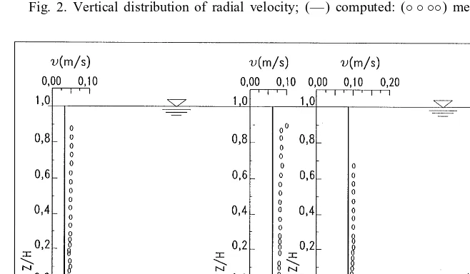
In Figs. 2 and 3, the comparison between numerical and experimental velocities is presented. A satisfactory agreement is achieved basically at any radial station, apart from the bottom boundary layer, where a small discrepancy is seen to occur. The ow eld is everywhere accelerated towards the discharging hole, particularly along the bottom oor. The bottom boundary layer is denitely conned, which means that it neither grows nor does it undergo any separation, as it has also been demonstrated experimentally [20]. Thus the vorticity produced at the boundary layer remains conned there.
Fig. 2. Vertical distribution of radial velocity; (—) computed: (◦ ◦ ◦◦) measured.
Fig. 3. Vertical distribution of tangential velocity: (—) computed: (◦ ◦ ◦◦) measured.
boundary layer would imply a massive renement of the mesh near the bottom; based on the above considerations, it was felt that such a mesh renement would introduce a great deal of complication that is, as a matter of fact, unnecessary. The numerical node nearest to the bottom was placed at 0.004 m from the oor, so that the simulation of the boundary layer was precluded.
6.1. The radial jet
The radial jet bears a strong resemblance to the Ekman layer that, however, occurs if all the experimental apparatus is forced to rotate (see, for instance, [15]). The Ekman layer was recognized as controlling the external vortex ow. Also, vortex circulation was found to be determined both by the owrate and by the Ekman layer depth [15].
Referring to the free surface vortex, Levi [11] was the rst researcher to discover the jet, as it was termed by the author, i.e., the fast owing uid along the bottom layer. This jet has much relevance in explaining the mechanism of vortex generation, that is based on momentum transfer between the jet and the overlying region of still uid.
Since vortex generation in a liquid is usually associated with the formation of a gradually deep-ening dimple that undergoes a progressive stretching, it is considered obvious that the vortex begins aloft and subsequently stretches downwards. Levi refutted this common belief and argued instead that the vortex should grow from below since the generating momentum comes from the under-lying jet. Actually, the very rst scientist who ventured in presenting this brilliant conjecture was Venturi (1797), cited by Levi [12], who stated: ...the rotation always begins and appears more
rapid in those parts of the uid closer to the bottom ... the funnel begins to form below : : : .
Levi’s hypothesis was conrmed by a simple experiment [20] consisting of injecting dye simulta-neously on the free surface and on the vertical axis of symmetry at a depth z≈0:6 H. The swirling motion was found to develop very quickly in the lower part, while at the same time the dye on the free surface remained perfectly still. Therefore, the vortex motion starts from below and cannot be seen from outside until the stretching of vortex line manages to reach the free surface, where the dimple is eventually generated.
The phenomenon described above is well simulated by the numerical model: in fact, after having attained the radial and vertical ow eld, the tangential velocity was imposed at the border. This tangential velocity propagates inside the domain and concentrates over the bottom hole, where it undergoes a huge amplication. Thisearly vortex, as it was speculated by Venturi (1797), Levi [11], and as seen experimentally by Trivellato [20], is stretched by the vertical component of velocity and propagates towards the free surface.
7. Conclusions
While the numerical model needs to be corroborated by more experimental data, according to the presented results (to be considered as yet as preliminary), it seems capable of reproducing the two most distinctive features of vortex motion, namely the azimuthal motion and the radial jet swiftly owing along the reservoir bottom.
Not only are Eqs. (1)–(4) valid for a laminar vortex, but they can also be accurate for turbulent vortices as well, since they are sucient to replace the kinematic viscosity = by the eddy viscos-ity . However, the value of is still a matter of speculation and no general consensus has been achieved so far.
A linear relationship, =k1 ∞, was rst postulated by Squire [19]. Referring to the decay of trailing vortices behind an aircraft, Scorer [18] proposed k1≈4·10−4
. Anwar [2] observed that the eddy viscosity for turbulent vortex ow should not be constant. Odgaard [17] estimatedk1≈6·10
As the last observation, the knowledge of the vortex far-eld circulation for a free surface vortex in an innite domain is only known from experiments; in fact, an analytical method for the a priori prediction of the circulation is currently not available.
Acknowledgements
This research received nancial support by the Ministry of University and of Scientic and Tech-nologic Research (funds M.U.R.S.T. 40%).
References
[1] H.O. Anwar, Coecients of discharge for gravity ow into vertical pipes, J. Hydraulics Res. 3 (1965). [2] H.O. Anwar, Turbulent ow in a vortex, J. Hydraulics Res. 7 (1969).
[3] D.N. Brocard, C.H. Beauchamp, G.E. Hecker, Analytic predictions of circulation and vortices at intakes, Electric Power Research Institute, Project 1199-8, Final Report, Palo Alto, California, 1982.
[4] V. Casulli, R.T. Cheng, Semi-implicit nite dierence methods for the three dimensional shallow water ow, Int. J. Numer. Meth. Fluids 15 (1992).
[5] R. Cola, F. Trivellato, Free surface vortex in an innite domain: the velocity representation, Idrotecnica 6 (1988). [6] L.R. Daggett, G.H. Keulegan, Similitude in free surface vortex formations, J. Hydraulics Eng. ASCE HY11 (1974). [7] H.A. Einstein, H. Li, Study vortex ow in a real uid, La Houille Blanche 4 (1955).
[8] R. Granger, Steady three dimensional vortex ow, J. Fluids Mech. XXV (1966).
[9] J.E. Hite, Vortex formation and ow separation at hydraulic intakes, Ph.D. Dissertation, Washington State University, Pullman, WA, USA, 1991.
[10] E. Kaasschieter, Preconditioned conjugate gradients for solving singular systems, J. Comput. Appl. Math. 24 (1988). [11] E. Levi, Experiments on unstable vortices, J. Eng. Mech. Div. ASCE 98 (EM3) (1972).
[12] E. Levi, The Science of Water, ASCE, New York, 1995.
[13] W.S. Lewellen, Three dimensional vortex ows, J. Fluids Mech. XIV (1962). [14] H.J. Lugt, E.W. Schwiderski, Birth and decay of vortices, Phys. Fluids 9 (1966).
[15] M. Mory, H. Yurchenko, Vortex generation by suction in a rotating tank, European J. Mech. B Fluids 12 (1993). [16] Y. Notay, Solving positive (semi)denite linear systems by preconditioned iterative methods, in: O. Axelsson,
L.Yu. Kolotilina (Eds.), Proc. Nijmegen The Netherlands, Lectures Notes in Mathematics, No. 1457, Springer, Berlin, 1989.
[17] A.J. Odgaard, Free surface air core vortex, J. Hydraulics Eng. 112 (1986). [18] R.S. Scorer, Local instability in curved ow, J. Inst. Math. App. 3 (1967).
[19] H.B. Squire, On the growth of a vortex in turbulent ow, Aero. Res. Counc., Paper n. 16666, London, 1954. [20] F. Trivellato, Free surface vortex in an innite domain, Ph. D. Dissertation, University of Padua, Italy, 1987. [21] F. Trivellato, On the near-eld representation in a free surface vortex, Proc. 12th Australasian Fluid Mechanics
Conf., vol a, Sydney, Australia, 1995.
[22] F. Trivellato, On the far-eld representation in a free surface vortex, Proc. 12th Australasian Fluid Mechanics Conf., vol. b, Sydney, Australia, 1995.