*Corresponding author.
Genetic algorithm optimisation of a class of
inventory control systems
S.M. Disney
*
, M.M. Naim, D.R. Towill
Logistics Systems Dynamics Group, Department of Maritime Studies & International Transport, University of Wales, Cardiw, P.O. Box 907, Cardiw, CF1 3YP UK
Received 16 March 1998; accepted 19 July 1999
Abstract
The paper describes a procedure for optimising the performance of an industrially designed inventory control system. This has the three classic control policies utilising sales, inventory and pipeline information to set the order rate so as to achieve a desired balance between capacity, demand and minimum associated stock level. A"rst step in optimisation is the selection of appropriate`benchmarkaperformance characteristics. Five are considered herein and include inventory recovery to`shockademands; in-built"ltering capability; robustness to production lead-time variations; robustness to pipeline level information"delity; and systems selectivity. A genetic algorithm for optimising system performance, via these"ve vectors is described. The optimum design parameters are presented for various vector weightings. This leads to a decision support system for the correct setting of the system controls under various operating scenarios. The paper focuses on a single supply chain interface, however the methodology is also applicable to complete supply chains. ( 2000 Elsevier Science B.V. All rights reserved.
Keywords: Inventory control; Optimisation; Simulation; Ordering algorithms
1. Introduction
Burbidge's Law of Industrial Dynamics states that`If demand is transmitted along a series of inventories using stock control ordering, then the amplitude of demand variation will increase with each transfera[1]. This results in excessive inventory, production, labour, capacity and learning curve costs, due to unnecessary
#uctuations in perceived demand [2]. One major cause is the time lag between a decision to make or order a unit of inventory and the realisation of that order [3]. It has long been understood (from knowledge of controller design), that the way to minimise this e!ect is to design the decision appropriately using control theory techniques to customise the response of the production/distribution decision [4]. This implies that the decision has a known structure and there are a number of such generic structures in use. A generic production/distribution control algorithm, termed the Automatic Pipeline Inventory and Order Based Production Control System (APIOBPCS) can be expressed in words as follows: `Production targets are
Nomenclature
¹M p production WIP gain.
u frequency (rads/time period)
APIOBPCS automatic pipeline, inventory and order based production control system.
AVCON average consumption
EWIP error in work in progress
ITAE integral of time*absolute error
ORATE order rate
PR robustness to production lead-time variations
s laplace operator, and (S) normalised Laplace operator
SV systems selectivity
t time
¹a consumption averaging time constant
¹i inverse of inventory based production control law gain
¹p production lag time constant
¹w inverse of WIP based production control law gain
WIP work in progress
WIPR robustness to pipeline level information"delity
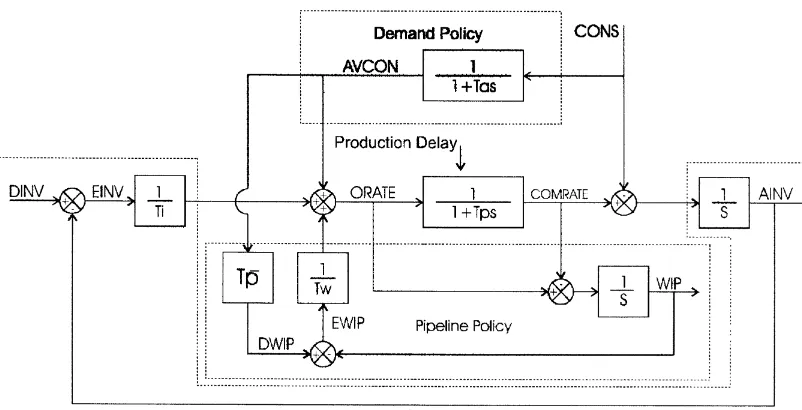
equal to demand averaged over¹atime units (the demand policy), plus a fraction,¹i, of the inventory de"cit in stores (the inventory policy), plus a fraction,¹w, of the WIP de"cit (the WIP policy)a. We usually express the model in continuous control form. However, the discrete version is also available, if preferred [5].
Fig. 1. Block diagram laplace representation of APIOBPCS.
Within the block diagram we have approximated the production delay in the Laplace domain by using 1/(1#¹ps/n)n, where n is either 1, for a "rst-order delay, or 3, for a third-order delay. Proof of this approximation is shown in [8]; and it is also thenth-order delay used in the DYNAMO/ STELLA/ iTHINK simulation packages [4]. It has been shown by various authors that these are good representation of real world production lead-time distributions, for example Wolstenholme [9].
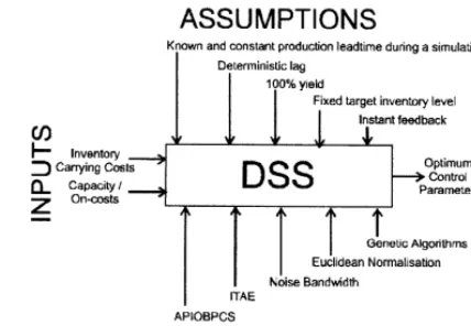
The focus of this paper will be to show how the control parameters,¹i,¹aand¹wchange as the balance between a situation's inventory carrying costs and production on-costs (capacity-related costs) alters. We will present a table of control parameters which re#ect various weightings on inventory and on-costs. To do this we will make extensive use of some control theory techniques coupled with an optimisation procedure termed, Genetic Algorithms (GA). As an aid to the structure and usefulness of the DSS and to the content of this paper, Fig. 2 shows the inputs, outputs, assumptions and tools and techniques that are used to develop the DSS.
2. Description of APIOBPCS
A description of the relevance of each policy element within APIOBPCS is now given [2].
2.1. Demand policy
Fig. 2. Outline description of the DSS.
smoothing, as it requires little data storage, is relatively accurate for short term forecasts, is a close approximation to the "rst order lag used in control theory and is readily understood. The question to be answered here is, how much weighting do we give to the recent demandxgures to attenuate theyuctuations in demand but at the same time respond to genuine changes?
2.2. Inventory policy
The inventory policy is to be considered because the rate at which we recover deviations in inventory will have a profound e!ect on production #uctuations [2]. It is often a misguided practice in industry that production targets are set to recover all the inventory de"cit in a single time period, even though it may take many more time periods for the product to be manufactured and appear in inventory holding [11]. This is continued for the whole of the production lead time. By the time the products begin to appear in the inventory there is signi"cant excess WIP on the shop#oor, which will inevitably increase the stock holding beyond the desired level. This will have to be reduced by producing less than the average market demand until the latter has reduced the inventory levels to the desired level. However, the same target overshoots happen here and the production rates are continuously #uctuating. As stock levels are related to our customer service levels and inventory o!sets result from decision making without explicit inventory policies, it is desirable to correct these discrepancies.The question to be answered here is, how much of the inventory discrepancy do we correct each time we set production/distribution requirements to avoid excessive overshoots and undershoots around the target level?
2.3. Pipeline policy
Fig. 3. The e!ect of the individual controllers on production order rates.
demand policies not considering the e!ects of the time delays in the system. It would then be bene"cial for the pipeline policy to reduce the production targets.The question to be answered here is, how quickly do we correct the pipeline deviation each time we set the production/distribution requirements?
2.4. The ewect of controller settings on system response
2.4.1. On the production orders
The e!ect of each controller in making up the production target (ORATE) is clearly shown in Fig. 3 [2] (a simulation model of APIOBPCS can be built in a spreadsheet environment using the di!erence equations shown in Appendix A). The smoothed sales signal (AVCON) is responsible for feeding forward the change from one level of sales to the other. The inventory feedback signal (EINV/¹i) is the main contributor to ORATE overshoot and oscillatory behaviour. The WIP signal (EWIP/¹w) is self adjusting, i.e. during times when WIP is too small it bolsters ORATE, and during times when WIP is too great it reduces ORATE. The e!ect of the WIP signal reduces the rise time of ORATE, and decreases the percentage overshoot; both favourable traits. However the downside costs must appear somewhere, which in this case is in the extended settling time. The more the emphasis given to the WIP feedback, the longer it takes to reach the steady state. This is due to the negative WIP signal cancelling out the inventory signal, thus giving more responsibility to the contribution of AVCON in reaching the steady state.
The problem can now be fully stated. We need to determine the optimum setting of the design parameters
¹a,¹iand¹w. An optimum setting of the parameters will:
f respond to genuine changes in demand quickly, f "lter out random noise in the sales pattern,
Fig. 4. The e!ect of¹a,¹wand¹ion inventory recovery following a step input.
practice is still di$cult [13]. It would therefore be bene"cial to consider the consequences of production variations on the dynamic response in our optimisation procedure, and thus ensure that the detrimental e!ects are minimised:
f be robust to delays in the WIP feedback loop as this information is not always easy to collect [12]. f be selective, in the sense that minor changes to the control parameters by real world users will not result in
signi"cant degradation of performance.
2.4.2. On the inventory levels
Fig. 4 shows the e!ect of the controller parameters on the actual inventory levels (AINV), following a step increase in sales from 100 to 200 widgets/time unit at time t"0. Each controller setting has been reduced by 25% of its nominal value. Decreasing ¹w will slightly reduce the maximum inventory de"cit, but it will take longer for the inventory levels to fully recover. Decreasing¹ahas a similar e!ect to¹i, but is less pronounced.¹iwill reduce the inventory freefall considerably more than reducing¹w
and the recovery is much quicker.¹ialso has the advantage over¹ain that after the freefall it is quicker in the recovery. However, too small a value of¹iresults in very poor "ltering properties in the presence of a random signal.
3. Performance characteristics of a scheduling algorithm
It is the aim of this section to highlight a method to determine how to judge the"tness of the values of the control parameters (¹i,¹aand¹w), for the"ve characteristics above. Summarising, the optimisation routine will assess the trade o!between:
f inventory recovery, f noise attenuation, f production robustness,
3.1. Quantixcation of characteristics
Each of the above"ve criteria for assessing the scheduling algorithms performance will now be quanti"ed to allow a GA to determine the"tness of a design, in order to optimise the scheduling algorithm. However,
"rst we will introduce the transfer functions of the system as these play an important role in the subsequent analysis. Then after the "rst two characteristics have been quanti"ed (inventory recovery and noise bandwidth) we will show some analysis to describe the nature of the basic trade-o!and the importance of the cost structure of real situations on the optimisation procedure. Finally, the remaining desirable character-istics will be described.
3.1.1. Transfer function analysis
By manipulating the block diagram in Fig. 1, a set of system transfer functions can be derived. Of particular interest is the ORATE/CONS and the AINV/CONS transfer functions, shown in Eqs. (1) and (2), respectively. The ORATE transfer function is useful as it yields information about the dynamic performance of the production targets and it plays an important role in de"ning the"ltering ability of the system. The addition of the WIP controller into the production control system has allowed us to de-couple the damping ratio from the natural frequency. This was not possible in the Inventory and Order Based Production Control System (IOBPCS) [14]. It also allows the"ltering characteristics of the system to be improved as the WIP controller forces the ORATE signal to be closer to the AVCON signal, at the expense of the inventory signal. The more the system is driven by the inventory signal the faster the system will become and the more reliant it is on the WIP controller to check its performance. Therefore, in these situations it is important that the WIP data acquisition system is operating, hence the WIP robustness performance vector.
ORATE
The AINV/CONS transfer function is useful because it gives information on the dynamic response of the inventory performance. The"nal value theorem can be applied to the AINV transfer function as shown in Eqs. (3) and (4). It shows us the importance of being able to accurately determine the production lead time. If an inaccurate production lead time has been used to set the desired WIP targets, then there is a permanent error in the steady-state inventory levels [6]. This is clearly jeopardising CSLs. Therefore, if a WIP controller is used to set production targets the lead time must be accurately known. It will be assumed in this paper that the lead time is known and constant throughout a particular simulation for the purpose of setting WIP targets only. This is representative of the real world scenario where companies monitor their lead time for setting WIP targets, but do not use it to update their optimum controller settings. It is all too often forgotten that the controller settings are a function of the production lead time [12].
The Final Value Theorem is given by
lim
t?=
Mf(t)N"lim
s?0
MsHf(s)N, (3)
wheref(s)"AINV/CONS, therefore in the limit
the"nal value"¹i
C
¹pN!¹p3.1.1.1. Inventory recovery. The integral of time*absolute error (ITAE) is generally agreed to be the most intuitive criterion following a step, for assessing transient deviations from a target. It is inevitable that a large error is present shortly after the step and it penalises more heavily, errors that are present later, by a suitable weighting in the time domain [15]. The ITAE also penalises positive and negative errors equally, and is the simplest measure that is reliable, applicable and selective [16].
The ITAE is de"ned in Eq. (5). Throughout this paper the ITAE was calculated following a step input in CONS that increased from 100 to 200 widgets per time period at time"zero:
ITAE"
P
0=
tDEDdt, (5)
wheretis the time period andDED the absolute error in inventory.
3.1.1.2. Noise attenuation. The ORATE noise bandwidth is important because it is a measure of the ability of the sales averaging time (¹a), time to adjust inventory (¹i), and time to adjust WIP (¹w), to"lter out the random higher frequency content of the demand, when setting production targets. The noise bandwidth is de"ned as the area under the system amplitude ratio squared curve [14]. For a linear system it is also proportional to the output variance. The noise bandwidth is a useful method of condensing frequency domain information into one criterion, and can be estimated from the frequency response plot. Alternatively it may be evaluated algebraically via Parsevals Theorem [17,18]. In the case of APIOBPCS for an assumed
"rst-order production lag the noise bandwidth equation is shown in Eq. (6) with the derivation later in Appendix B:
3.1.2. The nature of the trade-owand the importance of the cost structure
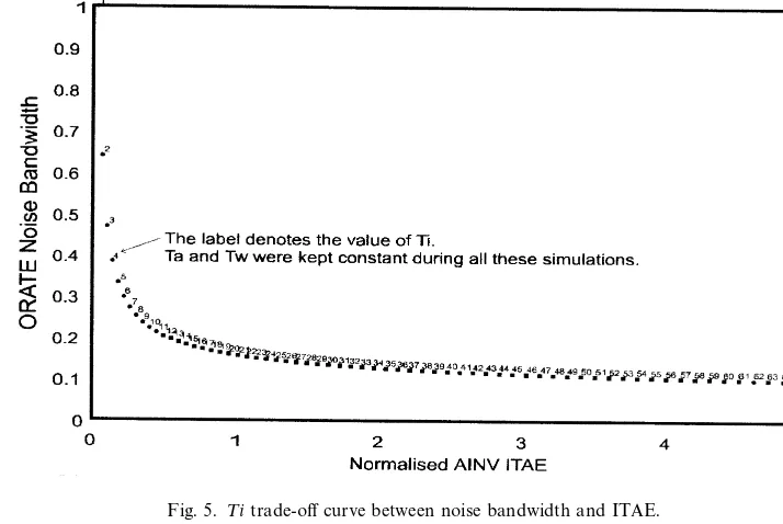
Fig. 5 below shows the nature of the trade-o!between the inventory recovery and noise bandwidth for a given set of control parameters (where¹aand¹wwere kept constant at 16 and 27 respectively, and¹iis changing). The inventory recovery has been scaled (divided by 1,600,000, a value determined via experi-mentation) so that its magnitude does not swamp out the noise bandwidth signal. With both vectors, the smaller the better, the optimum value of¹iis around 7. However, it can be envisioned that if the scaling factor on the ITAE value is reduced then the nearest point of¹ito zero increases.
Clearly, the scaling factor that should be used is dependant on the cost structure of the business involved. To determine the exact scaling factor an analysis of the inventory carrying costs and the production on-costs needs to be conducted. Therefore, for each situation there is a unique set of optimum control parameters, dependant on the scaling factor. Hence, the optimisation presented later determines the values of the control parameters based on weighting the inventory recovery and noise bandwidth criteria to re#ect the various cost structures that could be present.
Fig. 5. ¹itrade-o!curve between noise bandwidth and ITAE.
Fig. 6. Visualisation of the production robustness vector.
is based on the distance of the performance points from the centre of gravity. The centre of gravity is calculated by"nding the average ORATE noise bandwidth and the average ITAE. The spread is calculated using Euclidean normalisation, from Eq. (7). Appendix C lists the additional transfer functions used in the production robustness vectors.
PR"+pi/1+qj/1J[(ITAEij!+pi/1+qj/1ITAEij)/pq]2#[(uNij5691!+pi/1+qj/1uNij)/pq]2
where
PR"production robustness vector,
ITAE
ijis the ITAE for AINV under conditionsiandj(1)i)p), (1)j)q), wherep"q"3,
uNij"noise bandwidth of ORATE under conditionsiandj;
Conditionsi;
@i"1, production lag"4 time units,
@i"2, production lag"8 time units,
@i"3, production lag"12 time units,
@j"1, production lead-time distribution"exponential lag,
@j"2, production lead-time distribution"cubic lag.
3.1.2.2. WIP robustness. To reduce the order of the transfer function of an APIOBPCS model, a"rst-order lag is initially used to approximate a pure time delay in the WIP feedback loop. This is to simplify analysis. The purpose of this criterion is to establish the robustness of the design parameters to possible delays in the WIP feedback loop. Such delays as these may be present due to inaccuracies in the recording of WIP on the real world shop#oor. Like the production robustness vector and the selectivity vector the WIP robustness vector is a measure of how much the performance alters in the ITAE and noise bandwidth plane for all of the following conditions; No time delay; a"rst-order lag of 4 time units; and 8 time units. See Appendix B for the additional transfer functions required. It is de"ned as.
WIPR"+pi/1J[(ITAEi!+pi/1ITAEi)/p]2#[(uNi!+pi/1uNi)/p]2
p (8)
where
WIPR"WIP feedback delays robustness,
ITAE
i"the ITAE for AINV under conditionsi(1)i)p) wherep"3,
uN
i"noise bandwidth of ORATE under conditioni,
conditionsi;
@i"1, no WIP feedback delay,
@i"2, there is an exponential lag in the WIP feedback loop of 4 time units,
@i"3, there is an exponential lag in the WIP feedback loop of 8 time units.
100% and 125% of the nominal value and is calculated as follows:
i"noise bandwidth of ORATE under conditioni,
conditionsi;
3.1.2.4. Aggregation of the characteristics. The overall score assigned to a set of design parameters (¹a,¹i
and¹w) is now given by
SCORE" 1
JITAE2#u2
N#PR2#WIPR2#SV2
. (10)
The reciprocal has been introduced so that the higher the score, the better the dynamic performance of the ordering algorithm.
4. Optimisation of APIOBPCS via a genetic algorithm
technique for searching the solution space of problems that have many local minima, and adopted the idea for computer-based directed random searches.
GAs have two main areas of application [21], the"rst is the optimisation of the performance of a system, such as tra$c lights or a gas distribution pipeline system. They typically depend on the selection of parameters, perhaps within certain constraints, whose interaction restricts a more analytical approach. The second area of application for GAs is in the"eld of testing or"tting of quantitative models. In this case the aim of the GA is the minimisation of the error between the model and the data. The controller order reduction problem by Caponetto et al. [22]"ts this type of application. This paper is concerned with the"rst, i.e. an optimisation type application [23]. The GA approach was speci"cally used in this case due to its robustness to the possible shape of the solution space, the ease of implementation and acceptance as a good non-greedy searching mechanism.
4.1. The operation of the GA
LetXM"MxDx(L)
j )x)x(U)j N(1)j)M) be the search space whereMare the dimension ofxandx(L)j and x(U)
j the upper and lower limit of thejth componentxj of vectorx, respectively.
LetP(k)"Nbinary chromosome structuress
i(k) (1)i)N) in generationk.
Letf
i(k) be the"tness of the ith structure in generationkas de"ned by SCORE described earlier.
Letx
"(k) be the best parameter vector with the largest"tnessf"(k).
The GA works in the following way; Setk"0
Create initial random populationP(k)
Decodes
DO WHILEStermination conditions are not metT
Crossover and mutateP(k) to formN!1 chromosome structures and copy into populationP(k#1) Decoes
After convergence, the GA was restarted several times to check for the true optimum. In the description of the GA above¹pand¹M phave been set at 8 time units, the dimension ofx(M) is 3 (for¹i,¹aand¹w), and the upper and lower limit of eachxis 255 and 0, respectively. Thus the binary structures (s
i) are 24 bits long and
there wereN"60 binary chromosome structures.
4.2. Implementation of the optimisation procedure
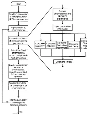
Fig. 7. Flow diagram of the simulation and optimisation procedure.
5. Optimum control parameters
Using the optimisation procedure outlined above the optimum control parameters such noise bandwidth and ITAE were given equal importance, i.e. the scaling factor on ITAE was 1,600,000, ¹a"
Table 1
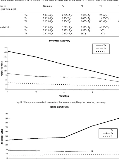
The optimum control parameters (¹w,¹aand¹i) for various weightings of the inventory recovery and noise bandwidth WeightingsN
Vector being weightedq
Nominal H2 H4 H8 H16
ITAE ¹w 5.125*¹p 4.375*¹p 3.375*¹p 2.5*¹p 1.5*¹p
¹a 2.125*¹p 1.75*¹p 1.625*¹p 1.625*¹p 1*¹p
¹i 0.875*¹p 0.75*¹p 0.625*¹p 0.5*¹p 0.5*¹p
Noise bandwidth ¹w 5.125*¹p 5.625*¹p 5.875*¹p 9.125*¹p 11.375*¹p
¹a 2.125*¹p 2.125*¹p 1.875*¹p 2*¹p 2*¹p
¹i 0.875*¹p 0.875*¹p 1*¹p 1*¹p 1*¹p
Fig. 8. The optimum control parameters for various weightings in inventory recovery.
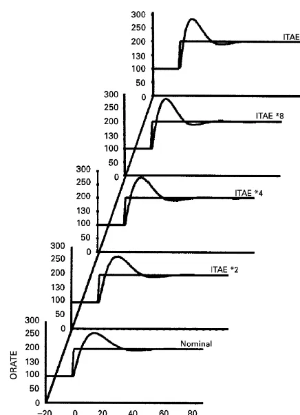
Fig. 10. Dynamic responses for the optimal ITAE weightings.
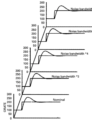
The dynamic performance of these optimal parameters when subjected to step input can be seen in Figs. 10 and 11 for the inventory recovery and the noise bandwidth weightings respectively, and similarly their response to a random demand is shown in Figs. 12 and 13.
6. Conclusion
Fig. 11. Dynamic responses for the optimal noise bandwidth weightings.
The optimisation procedure was then used to determine how the controller parameters would alter with di!erent cost structures within a production system. Considered was the weighting on inventory carrying costs and production on-costs or capacity costs re#ected in each of the"ve performance vectors. The set of controller parameters determined for the range of cost structures available ensures that users havea range of solutionsfor their business situation, thus forming a DSS. The DSS shows that as capacity costs become more important to a business (i.e. in process-oriented companies), the use of WIP information becomes negligible in the ordering decision, as ¹wbecomes very large. However, where inventory costs are signi"cant (i.e. in a batch/job shop oriented business) then WIP information has a considerable e!ect on the dynamic performance of the ordering system. Berry et al. [24] outlined similar results from an industrial survey of how WIP information is being used in practical situations. Their main conclusions show that companies with low and constant lead times (generally process type industries) were not collecting WIP information in their decision making and those that did (high, variable lead-time industries, i.e. jobshop type industries) could bene"t most from the inclusion of such information in their order decision making, but were failing to incorporate them formally in the feedback structure of the decision. This contribution suggests, that in industries where it is easy to collect WIP information, there is little bene"t in doing so. Conversely, where it is harder to collect WIP information there is considerable bene"ts to be obtained.
Fig. 12. Dynamic responses for optimal ITAE weightings to random demand.
improvement in dynamic performance in a three-level supply chain, for the nominal case, over and above the
`MRP equivalentacontroller settings of¹w"R,¹i"1 and¹a"0 [2].
Acknowledgements
The authors would like to thank the Royal Academy of Engineering for providing"nancial assistance via their International Travel Grant to present this paper at the 10th International Working Seminar on Production Economics.
Appendix A. Di4erence equations required for APIOBPCS
CONS
Parsevals relation, which for a third-order transfer function"(b22a
1/a3#b21!2b0b2#b20a2)/a2a1!a3
Therefore, the noise bandwidth equation for the ORATE/CONS with an exponential plant lag is
For a fourth-order transfer function, Parsevals relation becomes
b23
A
a1a2For a"fth-order transfer function Parsevals relation becomes [18]
1
Appendix C. Transfer functions required for APIOBPCS
C.1. APIOBPCS with axrst-order production lag,and axrst-order data collection lag in the WIP feedback path, ORATE transfer function
Note:¹q""rst-order lag constant in the WIP feedback path.
A.2. APIOBPCS with a third-order production lag,ORATE transfer function
References
[1] J.L. Burbidge, Automated production control with a simulation capability. Proceedings of IFIP Conference WG 5-7, Copenhagen, 1984.
[2] S.M. Disney, M.M. Naim, D.R. Towill, Dynamic simulation modelling for lean logistics, International Journal of Physical Distribution and Logistics Management 27 (3) (1997) 174}196.
[3] J.D. Sterman, Modelling managerial behaviour: Misconceptions of feedback in a dynamic decision making experiment, Manage-ment Science 35 (3) (1989) 321}339.
[4] J.W. Forrester, Industrial Dynamics, MIT Press, Cambridge, MA, 1961.
[5] K. Popplewell, M.C. Bonney, The application of discrete linear control theory to the analysis and simulation of multi-level production control systems, International Journal of Production Research 25 (1) (1987) 45}56.
[6] S. John, M.M. Naim, D.R. Towill, Dynamic analysis of a WIP compensated decision support system, International Journal of Manufacturing System Design 1 (4) (1994) 283}297.
[7] M.M. Naim, D.R., Towill, What's in the Pipeline? Second International Symposium on Logistics, 11}12 July 1995 pp. 135}142. [8] K. Chen, A quick method for estimating closed loop poles of control systems, Transactions of AIEE Applications and Industry 76
(1957) 80}87.
[9] E.F. Wolstenholme, System Enquiry: A System Dynamics Approach, Wiley, Chichester, 1990. [10] G. Stalk, T.M. Haut, Competing Against Time, Free Press, New York, 1990.
[11] D. Berry, D.R. Towill, Reduce costs*use a more intelligent production and inventory planning policy, BPICS Control (1995) 26}30.
[12] P. Cheema, Dynamic analysis of an inventory and production control system with an adaptive lead time estimator, Ph.D. Dissertation, University of Wales, Cardi!, 1994.
[13] J.M. Harrison, C.A. Holloway, J.M. Patell, Measuring delivery performance: A case study from the semiconductor industry, in: R.S. Kaplan (Ed.), Measures for Manufacturing Excellence, Harvard Business School Press, Boston, MA, 1990, pp. 314}321. [14] D.R. Towill, Dynamic analysis of an inventory and order based production control system, International Journal of Production
Research 20 (6) (1982) 671}687.
[15] D.R. Towill, Transfer function techniques for control engineers, ILIFFE Books Ltd, 1970, p. 52.
[16] D. Graham, R.C. Lathrop, The synthesis of optimum transient response: Criteria and standard forms. Transactions of the American Institute of Electrical Engineers, Applications and Industry 72 (1953) 273}288.
[17] P. Garnell, D.J. East, Guided Weapon Control Systems, Pergamon Press, Oxford, 1977, pp. 9}11.
[18] G.C. Newton, L.A. Gould, J.F. Kaiser, Analytical Design of Linear Feedback Controls, Wiley, New York, 1957, p. 372. [19] Darwin, C., The Origin of Species by Means of Natural Selection or the Preservation of Favoured Races in the Struggle for Life,
John Murrey, 1859.
[20] J.H. Holland, Adaptation in Natural and Arti"cial Systems, University of Michigan Press, Ann Arbor, MI, 1975.
[21] J.E. Everett, Model building, model testing, and model"tting, in: L. Chambers (Ed.), Practical Handbook of Genetic Algorithms, Applications, Vol. 1, CRC Press, Boca Raton, 1995, pp. 5}30.
[22] R. Caponetto, L. Fortuna, G. Muscato, M.G. Xibilia, Controller order reduction by using genetic algorithms, Journal of Systems Engineering 6 (2) (1996) 113}118.
[23] S.M. Disney, M.M. Naim, D.R. Towill, Development of a"tness measure for an inventory and production control system. Second International Conference on Genetic Algorithms in Engineering Systems: Innovations and Applications, University of Strathclyde, Glasgow, 2}4 September, 1997, IEE Conference Publication Number 446, ISBN, 0 85296 693 8, 1997b, pp. 351}356.
[24] D. Berry, G.N. Evans, and M.M. Naim, Pipeline control: A UK perspective, International Journal of Management Science, OMEGA 26(1) (1998), 115}131.