TEMPORAL CHANGES IN SEMIVARIOGRAM OF OCEAN SURFACE LATENT HEAT
FLUX UNDER LINEAR TREND
M. K. Singh∗
, P. Venkatachalam
CSRE, IIT Bombay, Powai, Mumbai, 400076 (manojks,pvenk)@iitb.ac.in
KEY WORDS:Temporal, Spatial, Statistics, Oceanography, Prediction
ABSTRACT:
One of the ways to study spatio-temporal variability of a process is to consider it as a temporal variation of a spatial process. Semivar-iogram is a measure of spatial variation in a process. If a process is undergoing a linear trend, then semivarSemivar-iogram parameters such as range, sill and nugget are bound to change. In this paper, a mathematical closed form of range, sill, and nugget and in turn semivari-ogram were expressed for a process under linear trend. The derived semivarisemivari-ogram was used to study the latent heat flux (LHF) over the Indian Ocean. LHF values depend on sea surface temperature (SST) and wind speed (WS) over ocean surface. Universal kriging (UK) was used to estimate the LHF with WS and SST as covariables. UK coefficients corresponding to covariables were found out for the years 2010, 2020, 2030, 2040 and 2050. In similar line, study has been attempted to see how empirical orthogonal function modes of a spatio-temporal process change with time under linear trend.
1. INTRODUCTION
There are several ways to interpret a spatio-temporal process. The process can be thought as a spatial process which evolves with time. Study of the spatial behavior of the process with time is important in many fields. As an example, temporal behavior of LHF with respect to changes in WS and SST was considered in this paper. Study of LHF is important as it is a key component of hydrological cycle. In recent decades signification positive trend in LHF of World Ocean was observed. WS and SST values have also increased in recent times. Therefore study of LHF along with WS and SST is interesting (Li et al., 2011). Universal kriging method was used in this study, to relate LHF with their covari-ables. Kriging coefficients and their variances can be computed using equations UK systems of equation. The UK coefficients determine the contribution of WS and SST on LHF. The variance of the parameters determine their reliability. It will be interesting to see how these coefficients change and their variances change with time. Therefore, the problem statements are
1. Letβ0,V(β0),βkandV(βk)represent the UK coefficient
vector and the variance matrix at timet= 0and at timet=
krespectively. Then givenβ0andV(β0)can we estimate βkandV(βk)?
2. If we know the semivariogramγ0 at timet = 0, can we estimate semivariogramγkat timek
This work was centered towards studying these problems under assumption that the process and its covariates have linear trend. Temporal behavior of semivariogram is discussed in next section and the results related to temporal changes in UK coefficients and their variances are discussed in section 3.. More about universal kriging can be found in (Chiles and Delfiner, 2009)
2. METHODOLOGY
At timet= 0, the LHFY0(s)is given by
Y0(s) =µ(s) (1)
∗
Corresponding author.
If we assume LHF has annual trendωl, then, afterkyears, LHF
will be,
Yk(s) =µ(s) +ωl(s)×k (2)
Trends can also be considered as a spatial process. Let us denote γ(h)as the semivariogram of LHF trend. Then,
γk(h) = 1 2N
X
s
yk(s+h)−y(s)2 (3)
= 1
2N
X
s
µ(s+h) +ωl(s+h)×k−µ(s)−ωl(s)×k2(4)
= 1
2N
X
s
n
[µ(s+h)−µ(s)]2+k2
ωl(s+h)−ωl(s)2o(5)
= γ0(h) +k2γ(h) (6)
the non-square term not shown in equation 5 is sum of equal but opposite numbers and hence zero. In equation 6,γk(h)increases
as kincreases. Sinceγ0(h) >> γ(h), for small values ofk, spatial variability does not change significantly. As time changes significantly i.e. kis large enough,k2γ(h)cannot be neglected fromγ(h). For the purpose of this study we assume that semivar-iogram is a continuous function ofh, with a possible exception ath= 0. Forhgreater than a distance, called as range, semivar-iogram is constant. From equation 5, it is easy to conclude that, the range ofγk(h)will be maximum of the range ofγ0(h)and
γ(h). SillSkofγk(h)will be given by,
Sk=S0+k2×S (7)
whereS0is sill ofγ0andSis sill ofγ. Once range and sill are known, closed form of semivariogram can be found.
Kriging system of equation can be solved using variance covari-ance matrix, instead of semivariogram. Properties of varicovari-ance similar to that in the equation 6, can also be developed. Ifγand covariance functionCare continuous function ofh, then
lim
h→∞
γ(h) = C(0)− lim h→∞
C(h) (8)
lim
h→∞
γ(h) = C(0) (9)
In practice we assume γ(h) to be constant for hgreater than range. Therefore, varianceC(0)can be written as semivariogram of largeh. LetC0(h)andCk(h)be variance at timet= 0and The International Archives of the Photogrammetry, Remote Sensing and Spatial Information Sciences, Volume XL-8, 2014
ISPRS Technical Commission VIII Symposium, 09 – 12 December 2014, Hyderabad, India
This contribution has been peer-reviewed.
timek= 0. If the process is second order stationary, then
Ck(h) = Ck(0)−γk(h) (10)
= γk(R)−γk(h) (11)
= γ0(R) +k2γ(R)−γ0(h) +k2γ(h) (12)
= γ0(R)−γ0(h) +k2(γ(R)−γ(h)) (13)
= C0(0)−γ0(h) +k2[C(0)−γ(h)] (14)
= C0(h)−k2C(h) (15)
whereRis the maximum of the ranges ofγ(h)andγ0(h). The covariance matrix at timetcan be written as
Σ(ˆk)
β = (B
(k)T
n V
−1 (k)B
(k)
n )
−1
(16)
and calculated coefficient vectorβˆwill be given as,
ˆ
β(k)= Σ(βˆk)B (k)T
n V
−1 (k)Z
(k)
n (17)
whereBnis a matrix of sizen×3, first column of which is filled
with1, second column represents wind speed trend and third col-umn represents SST trend fornlocations. Zn(k) represents true
LHF at timek.
To establish a relationship betweenΣ(ˆk)
β andΣ
(r) ˆ
β and between
ˆ
β(k) andβˆ(r), we need to know relationship betweenB(
k)
n and
Bn(k)and betweenZ( k)
n andZ( r)
n . It is not an easy task to
estab-lish such relationships. Nevertheless, we can still be able to find
Σ(ˆk)
β andβˆ(k)by direct calculations. The results related to direct
computation of universal kriging of LHF with WS and SST as co variables are summarized in the next section.
3. RESULTS AND DISCUSSION
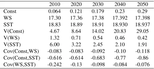
Table 1 shows the UK coefficients, their variance and covariance.
2010 2020 2030 2040 2050
Const 0.064 0.121 0.179 0.23 0.29
WS 17.30 17.36 17.38 17.392 17.398
SST 18.83 18.89 18.91 18.930 18.937
V(Const) 4.67 8.64 14.02 20.83 29.05
V(WS) 1.32 0.71 0.54 0.46 0.42
V(SST) 6.00 3.22 2.45 2.10 1.91
Cov(Const,WS) -0.083 -0.083 -0.092 -0.10 -0.118 Cov(Const,SST) -0.616 -0.614 -0.683 -0.77 -0.86 Cov(WS,SST) -0.242 -0.13 -0.098 -0.084 -0.076
Table 1: UK coefficients and their variability expected in coming decades
Following observations can be interpreted from the table:
1. Contribution from parameters other than WS and SST in-creases with time, although the contribution is small as com-pared to WS and SST. The variance of factors other than WS and SST increases very fast and therefore their reliability de-creases with time.
2. WS and SST coefficients increase at a very small rate but their variances decrease very quickly. Therefore, their relia-bility increases with time. In most of the regions LHF, WS and SST have positive trend. Therefore, it is expected to find increment in the UK coefficients.
3. The three variables are negatively correlated. Correlation between WS and SST with other parameters increases with time but between WS and SST decreases.
ACKNOWLEDGEMENTS
The authors thank INCOIS, Hyderabad team for providing the data set of latent heat flux, wind speed and sea surface tempera-ture
REFERENCES
Chiles, J.-P. and Delfiner, P., 2009. Geostatistics: modeling spa-tial uncertainty. Vol. 497, John Wiley & Sons.
Li, G., Ren, B., Yang, C. and Zheng, J., 2011. Revisiting the trend of the tropical and subtropical pacific surface latent heat flux during 1977–2006. Journal of Geophysical Research 116(D10), pp. D10115.
The International Archives of the Photogrammetry, Remote Sensing and Spatial Information Sciences, Volume XL-8, 2014 ISPRS Technical Commission VIII Symposium, 09 – 12 December 2014, Hyderabad, India
This contribution has been peer-reviewed.