ASSESSING TEMPORAL BEHAVIOR IN LIDAR POINT CLOUDS OF URBAN
ENVIRONMENTS
J. Schachtschneider∗, A. Schlichting, C. Brenner
Institute of Cartography and Geoinformatics, Leibniz Universit¨at Hannover, Germany - (julia.schachtschneider, alexander.schlichting, claus.brenner)@ikg.uni-hannover.de
KEY WORDS:LiDAR, Mobile Mapping, Alignment, Strip Adjustment, Change Detection
ABSTRACT:
Self-driving cars and robots that run autonomously over long periods of time need high-precision and up-to-date models of the changing environment. The main challenge for creating long term maps of dynamic environments is to identify changes and adapt the map continuously. Changes can occur abruptly, gradually, or even periodically.
In this work, we investigate how dense mapping data of several epochs can be used to identify the temporal behavior of the environment. This approach anticipates possible future scenarios where a large fleet of vehicles is equipped with sensors which continuously capture the environment. This data is then being sent to a cloud based infrastructure, which aligns all datasets geometrically and subsequently runs scene analysis on it, among these being the analysis for temporal changes of the environment.
Our experiments are based on a LiDAR mobile mapping dataset which consists of 150 scan strips (a total of about 1 billion points), which were obtained in multiple epochs. Parts of the scene are covered by up to 28 scan strips. The time difference between the first and last epoch is about one year. In order to process the data, the scan strips are aligned using an overall bundle adjustment, which estimates the surface (about one billion surface element unknowns) as well as 270,000 unknowns for the adjustment of the exterior orientation parameters. After this, the surface misalignment is usually below one centimeter. In the next step, we perform a segmentation of the point clouds using a region growing algorithm. The segmented objects and the aligned data are then used to compute an occupancy grid which is filled by tracing each individual LiDAR ray from the scan head to every point of a segment. As a result, we can assess the behavior of each segment in the scene and remove voxels from temporal objects from the global occupancy grid.
1. INTRODUCTION
It is nowadays agreed upon that self-driving cars will need highly accurate maps for their reliable operation. However, since the en-vironment undergoes temporal changes, the usefulness of a map is dependent not only on its geometric accuracy, but also on its ability to represent the current state of the scene. Unfortunately, many scene parts in the vicinity of roads change quite frequently. For example, a new object may appear in the environment and stay there permanently, like a new building, or it can stay only temporally, like a parked car. Objects can move or change their appearance, like open or closed gates or doors. Surfaces can wear off and vegetation will continuously grow until it is cut back or changed otherwise due to seasons.
One solution to this problem would be a very dense sampling (in time) of the scene, so that all temporal changes are faithfully represented in the map. As this approach is not economically viable, one can instead rely onknowledge about the scene and its temporal behavior, in order to assess its current state. This is similar to the approach that humans take. For example, one would usually expect buildings to be static, so they can be used as landmarks. On the other hand, we would not include parked cars when giving directions. In order to mimic this behavior, the first step is to understand the different parts of a scene, in terms of a classification into certain behavioral classes, which are then attached to the map. As a result, a robotic system (such as a self-driving car) which intends to interpret the scene contents with the help of this map will be less ‘surprised’ by scene changes if they are to be expected anyways.
∗Corresponding author
Reviews on recent methods for change detection and deformation analysis, e.g. (Lindenbergh and Pietrzyk, 2015, Qin et al., 2016), identify that most approaches for change detection in urban envi-ronments are based on airborne data using Digital Surface Models (DSMs). The traditional change detection methods (especially in airborne laser scanning) compare point clouds themselves and do not use the additional information of the sensors position during measurement. (Girardeau-Montaut et al., 2005) compare popular state-of-the-art distance based strategies. They identify that using the Hausdorff distance leads to much better results than average distance or using a best fitting plane.
(Kang and Lu, 2011) use the Hausdorff distance to detect changes in point clouds of urban environments obtained by static terres-trial laser scanners. They are motivated by disaster scenarios like earthquakes or floods where the changes in densely populated urban areas shall promptly be detected in order to speed up the emergency response. Accordingly, they focus mainly on disap-pearing changes in building models. They use the scale invari-ant feature transform (SIFT) method to align point clouds from multiple measurements and then use the Hausdorff distance to compute changes between the different measurement epochs. In order to analyze the resulting point segments marked as changed, they compute planar surface areas and provide those for damage estimation.
(Hebel et al., 2013) present a framework to compare current aerial laser scan data of an urban environment to a reference on-the-fly. After they align the actual measurement with the reference, the resulting point cloud is analyzed pointwise using Bresenham’s algorithm (Bresenham, 1965) for ray tracing. The space between the sensor head and a reflecting point is determined as empty and the unseen space behind this point is unknown as long as it is not determined by another scan ray. In contrast to distance based methods, this approach can handle occlusion. The transition be-tween different states (empty to occupied, occupied to unknown) is modeled smoothly by a belief assignment to points in the laser beam. In order to avoid conflicts with rays crossing penetrable objects, they pre-classify vegetation before alignment and model it with different parameters.
The approach of (Xiao et al., 2015) applies the above mentioned method to laser scan data from mobile mapping. They model the laser beam as a cone in order to improve the ray tracing results. In contrast to (Hebel et al., 2013) they do not use pre-classification, but avoid conflicts with penetrable objects by combining their method with a point-to-triangle distance based change detection. As a result of their method they mark points as uncertain, con-sistent and conflicting. In a comparison of different change de-tection methods (occupancy-based, occupancy-based with point normals, point-to-triangle-based, combination) they show that the combined method takes advantages of both, distance-based meth-ods and occupancy grids. It is robust with penetrable objects and can deal with occlusions.
(Aijazi et al., 2013) use multi-temporal 3D data from mobile mapping and presented an approach that not only detects but also analyses changes in an urban environment. In order to deal with occlusion, they first segment the point clouds and then classify objects as permanent or temporal using geometrical models and local descriptors. Afterwards they remove the temporal and all unclassified objects from each point cloud of the single measure-ments and then match the remaining points using the ICP (iter-ative closest point) method. That way they fill holes caused by occlusion from now removed temporal objects. They map the resulting clouds into 3D evidence grids and compare those (al-ways the actual versus the previous measurement) to update their similarity map by using cognitive functions of similarity.
In contrast to existing approaches, we do not only want to de-tect changes in the map but also classify them into distinct types, according to their behavioral patterns.
2. DATA
For our experiments we used data acquired by a Riegl VMX-250 Mobile Mapping System, containing two laser scanners, a cam-era system and a localization unit (figure 1).
The localization is provided by a highly accurate GNNS/INS sys-tem combined with an external Distance Measurement Instru-ment (DMI). The preprocessing step is made using proprietary Riegl software and additional software for GNSS/INS process-ing, using reference data from the Satellite Positioning Service SAPOS. The resulting trajectory is within an accuracy of about 10 to 30 centimeters in height and 20 cm in position in urban areas. Each scanner measures 100 scan lines per second with an over-all scanning rate of 300,000 points per second (RIEGL VMX-250, 2012). The measurement range is limited to 200 meters, the ranging accuracy is ten millimeters. For this experiment, we used data from six measurement campaigns in Hannover-Badenstedt
Figure 1. Riegl VMX-250 placed on a Mobile Mapping van.
Figure 2. Measurement area in Hannover-Badenstedt (Germany). The scan points are colored by the maximum height
difference in every grid cell, from blue (0 cm) to red (2 cm).
(Germany), which took place on 4.7.2012, 30.1.2013, 4.4.2013, 18.4.2013, 2.7.2013, and 20.8.2013. From all campaigns, we used only scan strips which overlap a small area of four blocks of buildings, shown in the center of Figure 2. The horizontal ex-tent of this figure is 1.4 km, the central part of the four blocks of buildings has an area of about 0.5×0.5 km2. The resulting point cloud consists of 1.48 billion points.
3. ALIGNMENT
In order to assess temporal changes between different measure-ment campaigns, the data has to be in the same global coordi-nate system. The absolute accuracy is governed by the position and orientation determination of the van, which is tied to the GNSS/IMU system. As mentioned above, depending on GNSS conditions, errors in the range of several decimeters can be ob-served. In contrast, the accuracy of the laser range measurement as such is about one centimeter (with contemporary systems even better, 5 mm accuracy, 3 mm precision), which is about two mag-nitudes better.
0.1 mgon angle measurement accuracy), resulting in maximum standard deviations of 1.1 mm in position and 1.3 mm in height for the network points. Global referencing was done using a GNSS survey (6.6 mm accuracy). Based on the geodetic network, free stationing was used to determine the position and orientation of a total station, which was in turn used to measure the final con-trol points of the testfield (2 mm + 2 ppm distance, 0.3 mgon an-gle accuracy). Overall, 4,000 individually chosen points on build-ing facades and additional (automatically measured) profiles on the road surface were measured. Such data can be used to align scan data globally, however the effort to obtain it makes it not practicable for larger areas.
Therefore, one has to settle for less costly methods, one of them being the alignment of all scan data with each other. This is a very well-known and well-researched topic. In case of aligning multi-ple individual datasets, theiterative closest pointalgorithm (Besl and McKay, 1992, Rusinkiewicz and Levoy, 2001, Segal et al., 2009) is normally used to iteratively minimize the point or sur-face distances. In case of measurements obtained from a moving platform, the problem is known in robotics asSLAM (simultane-ous localization and mapping, (Grisetti et al., 2010)), while, es-pecially in the scanning literature, it is known asstrip adjustment
(Kilian et al., 1996). For platforms which capture data continu-ously, it is usually formulated in terms of a least squares adjust-ment which estimates corrections for the position and orientation at constant time or distance intervals along the trajectory (Glira et al., 2015).
In simple cases, the adjustment can be formulated in terms of minimizing the pairwise distance between scan strips. However, when a lot of scan strips overlap (e.g. in our test area, there are up to 28 scan strips at certain locations), forming all possible pairs is not feasible, as this grows quadratically (in the number of scan strips). Instead, the usual approach is to introduce the surface in terms of additional unknowns, similar to using tie points in pho-togrammetry. Then, the problem grows only linearly in the ber of scan strips, however, at the cost of introducing a large num-ber of unknowns required to describe the surface. The geometric situation is depicted in figure 3, where blue and green are two trajectories from different scan strips,a1, . . . , a3andb1, . . . , b3 areanchor pointswhere corrections to the exterior orientation are estimated for the blue and green trajectory, respectively, andmis a single surface element whose distance to the measured points is observed.
b
b2 b3
b1
a1 a2
a3 m
Figure 3. Geometric situation for the example of two scan strips. Blue and green curves are trajectories of the mapping van, red
lines are scan rays,aiandbiareanchor points(where
corrections for the exterior orientation are estimated), andmis one single surface element, where scan points are assumed to
align.
In order to formulate this as a global adjustment model, three
equation types are needed:
1. Measured points (red rays in figure 3) which are assigned to a surface elementmshall coincide with the surface,
2. the original trajectories shall not be modified (forcing the corrections in the anchor points to be zero), and
3. successive corrections in anchor points (e.g., froma1toa2) shall be the same,
where all these conditions are to be enforced with appropriate weights. Then, adjustment can be used to minimize both, the an-chor points and the surface model, in one global, monolithic min-imization procedure. Unfortunately, the number of unknowns is very large in this case. For example, for the Hannover-Badenstedt test scene, there are 278,000 unknowns for the anchor points, but almost one billion unknown surface elements (when a local sur-face rasterization of 2 cm is used).
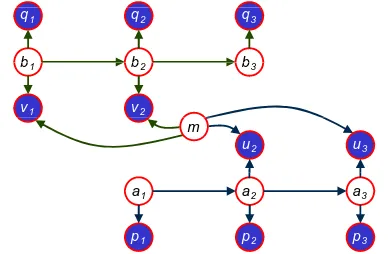
Figure 4 shows the Bayes network resulting from the situation in figure 3 and the equation types (1)-(3). The global minimization would require to compute
ˆ
A,Mˆ = arg max A,M
Ω (A, M) (1)
whereAandMdenote the unknown anchor points (in the exam-ple,a1,a2,a3,b1,b2,b3) and surface elements (m), respectively, andΩis the target function, usually formulated in terms of a least squares error. However, a na¨ıve implementation leads to equation systems of intractable size, which grow mainly with the overall size of the scene.
b b b
q1 q2 q3
b1 b2 b3
v1 v2
u2 u3
m
a1 a2 a3
p1 p2 p3
Figure 4. Bayes network for the situation in figure 3.ai,biand
mare the unknowns for the anchor points and surface elements, respectively,ui,viare the observed distances from the measured
points to their assigned surface element (equation type 1), and pi,qiare the observed exterior orientations (equation type 2).
Equation type 3 results in conditions between successive unknowns (ai,ai+1andbi,bi+1).
which is even more simple. This leads to the followingalternate least squares approach, which, instead of optimizing eq. 1, alter-nates the two steps
ˆ
A= arg max A
Ω (A, M) and
ˆ
M= arg max
M
Ω (A, M).
In (Brenner, 2016), this approach is described in more detail and the mapping of the computational process to a standard ‘big data’
MapReduce approach is shown. The global adjustment leads to standard deviations below one centimeter for the surface el-ements. After adjustment of all anchor points, the point cloud is recomputed globally, which then forms the input to the subse-quent change detection.
4. CHANGE DETECTION
Changes in urban environments may be caused by several rea-sons: pedestrians on the sidewalk, moving or parked cars, con-struction sites or even changing vegetation. We do not only want to detect these dynamics in the data but also analyze the various behaviors of different objects in the environment.
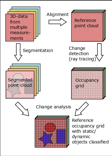
Our change detection method consists of four main steps (see fig-ure 5): First, all measfig-urements are aligned into a reference point cloud. Second, all point clouds from different measurement runs are segmented. Afterwards, all points of the reference point cloud are accumulated into an occupancy grid. Finally, the occupancy grid is combined with the segmentation results and stored as a reference grid.
3D-data from multiple measure-ments
Reference point cloud
Segmentation
Change analysis Change detection (ray tracing)
Reference occupancy grid with static/ dynamic objects classified Alignment
Segmented point cloud
Occupancy grid
Figure 5. The four main steps of our change detection method: alignment, segmentation, change detection and change analysis.
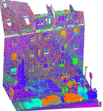
After the alignment described in the previous section, we seg-mented the occurring objects in the point clouds. We used a re-gion growing algorithm (Adams and Bischof, 1994) to remove the ground. After choosingnseed points, which in this case are
the points with the lowest height values, we compared the neigh-bouring points using the distance to the current region and the local normal vectors and removed the corresponding points from the point cloud. In a further step, we again used a region grow-ing algorithm, applied to the remaingrow-ing points, to find connected objects. An example result can be seen in figure 6.
Figure 6. Result of the region growing algorithm. Each connected object is assigned a random color.
In the next step, we computed 3D occupancy grid maps from the point clouds. We divided the space into voxels with an edge length of ten centimeters. The analysis principle can be seen in figure 7. As we know the trajectory of each laser scanner head, we can trace the laser beam for every single measured point. We used the voxel traversal algorithm presented by Amanatidis and Woo (Amanatides et al., 1987). A voxel is free, if it does not con-tain any reflecting points and the laser beam passes through the voxel on its way from the laser scanner head to an occupied voxel. If on the other hand at least one reflecting point falls into a voxel, it is marked as occupied. Voxels which are never crossed and contain no points are marked as unseen. This analysis is done for every point cloud of several measurement runs and the status of every voxel is stored in the occupancy grid of the corresponding run. In the following, the three possible voxel states are encoded as “free” (0), “occupied” (1), and “unseen” (2). For each single voxel, the sequence of measurement runs results in a sequence of such codes, which represent the behavior pattern of each voxel. E.g. if a static object is permanently part of the scene, its behav-ior pattern will constantly have the state “occupied” and an object that disappears after some time will have a falling edge from “oc-cupied” to “free” in its state sequence. Using this state sequence, the behavior of every voxel can be evaluated in the final change analysis step.
1/1
1/1
1/1 1/1
1/1 1/1
1/1
1/1 1/1 1/1 1/1 1/1 1/1 1/1 1/1 1/1
1
(a) 1strun.
1/4
3/4 3/4 3/4
3/4 3/4
1/3 1/3 1/3
1/3 1/3
1/4
4/4 4/4
4/4 4/4 4/4 4/4 4/4 4/4 4/4 4/4 3/3 3/3
4
(b) 4thrun.
1/8
3/8 3/8 3/8
3/8 3/8
6/8 6/8 5/7
6/8 5/7
1/8
8/8 8/8
8/8 8/8 8/8 8/8 8/8 8/8 8/8 8/8 6/6 7/7
8
(c) 8thrun.
Figure 7. Illustration of voxel counting. On its way along the trajectory, the laser scanner (red) on the vehicle (yellow) permanently scans its environment. If the laser beam is reflected by an object, e.g. a building facade (green), the corresponding voxel count in the
occupancy grid increases. The first value in the voxels indicates how often the laser beam hits the voxel, the second value how often the voxel was visible (i.e., the laser beam hits or crosses the voxel). The pedestrians (orange) have only been seen once. The parked cars (blue) on the street have been seen in three or six of eight measurements. Voxels to the right of the red beam are yet to be scanned.
pattern, in the previous step. Counting unique patterns results in the “number of patterns” column in table 1.
Figure 8. Point cloud consisting of multiple scans, using a random color for each scan.
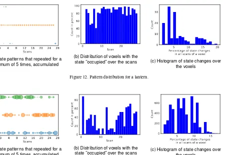
Figure 9 shows a histogram of the patterns of the lantern, which covers 152 voxels, resulting in 89 unique patterns (sorted in as-cending frequency). The shape of the histogram is quite common to all objects and shows that only a few patterns occur most fre-quently and define the overall behavior of an object. Thus, for further analysis, we keep only voxels which exhibit patterns that occur at least five times (in the respective object). The distri-bution of the (remaining) patterns over all scans are shown in figures 11a – 15a (notice that the measurements are not equally distributed in time). Here, the horizontal axis enumerates all (28) scans, the vertical axis is the state (0, 1, 2, encoding “free”, “oc-cupied”, and “unseen”), and the size of the markers encodes the frequency.
The patterns show that the state of the voxels in static objects (like the facade, the lantern and the bush) are almost constantly occu-pied. While for a relatively small and geometrical simple object
Observed objects No. of No. of Final voxels patterns state
facade 6484 5168 p
lantern 152 89 p
bush 5693 4894 p/ t
hedge 446 414 p/ t
parked vehicle 1 733 463 t parked vehicle 2 665 384 t parked vehicle 3 358 266 t
motorbike 421 301 t
pedestrian 1 97 57 t
pedestrian 2 106 36 t
Table 1. Observed objects for state pattern analysis, final state expected to be permanent (p) or temporal (t).
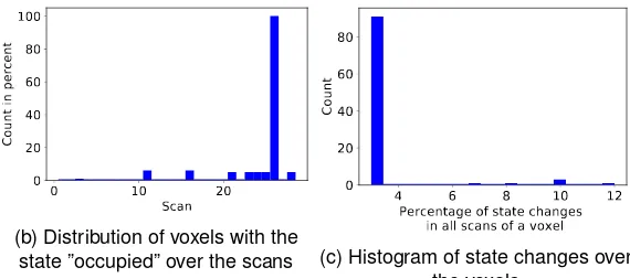
like a lantern, only a few false detections of free voxels occur, for larger and more complex objects like the facade, this propor-tion is larger. For vegetapropor-tion, like the bush, the state toggles even more often between occupied and (false) free. As mentioned be-fore, this behavior of vegetation can have different reasons like growth, seasonal changes, human intervention, and the penetra-bility of the object. The car appeared in the scene at the 5th mea-surement and stayed there until the end. The pedestrian was only scanned once in measurement run 24.
Figures 11b – 15b show how many voxels are occupied in every scan of an object. These match the behavior patterns in figure 11a – 15a. They show that for vegetation, in total less voxels are occupied over the scans than in the other static objects. Further-more, vegetation has a lot more state changes over the different measurement runs than other static objects, as shown in figure 11c – 15c .
0 20 40 60 80 Patterns
0 5 10 15 20
Count
Figure 9. Frequency of the behavior patterns of a static object (lantern).
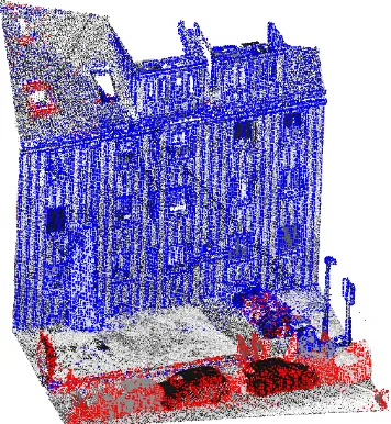
Figure 10. Point cloud after change detection; blue: permanently occupied, red: temporarily occupied
at least 25% of all voxels in a segment are occupied in at least 70% of all measurements, the object is assumed to be permanent.
Based on this threshold we started to define the final states of the objects. We considered three different states: “permanently occupied”, “temporarily occupied”, and “free”. Typical objects for the expected states are shown in table 1.
All voxels of a segment are rated as permanently occupied if at least 25% of all voxels in that segment are occupied in at least 70% of all measurement runs and rated as temporarily occupied if less than 25% of all voxels in that segment are occupied in 70% of all measurement runs. The rest of the seen voxels is rated as free. Once the final states of all objects are determined, the corresponding voxels in the global grid are updated. As a result, we obtained a voxel grid with a defined final state for each voxel. Figure 10 shows the result of the change detection and analysis in a typical street scene.
5. RESULTS AND DISCUSSION
As shown in figure 10, permanent static objects like facades, lanterns and parts of the vegetation are separated from objects that appear only temporarily like pedestrians and parked cars. How-ever, some parts of vegetation are also considered as temporarily and some pedestrians are considered as permanent. These false permanent detected pedestrians may be caused by a too coarse segmentation where the pedestrians are merged with some static parts of the environment into one object. Since the pedestrians are represented by relatively few points, their proportion in a false-merged segment is relatively low, and the static part of the false-merged segment will dominate. This could be avoided by a finer segmen-tation. Or, since we take into account multi-temporal measure-ments, we can avoid this by comparing the extent and overlapping of different segments from different timestamps. Vegetation is sometimes considered as temporal because of two main reasons, one is its permeability and the other one is that it changes over time (due to growth, seasonal changes or human interventions). For a more accurate change detection the behaviour patterns of vegetation from a wider change analysis could be considered or vegetation could be classified in advanced.
Another drawback of our method is that we classify the states by counting the occupied voxels and calculate their proportion of space (segment) and time (measurement runs). This means we would still detect an object that has been part of the environment for a long time and was recently removed as permanent. This could be avoided by taking into account the state patterns of the temporal objects and e.g. detect a falling or rising edge for objects that are added or removed.
6. CONCLUSION AND OUTLOOK
In the future, we want to analyze the change patterns of different objects more precisely and classify changes in more detail, e.g. take into account the lifetime of an object and detect falling or rising edges in their state patterns, so we can add or remove them from the reference grid. In addition, we want to classify objects by their typical behavior in order to estimate their “probability to change” and add these information to the global map. Therefore, we want to add a classification step to improve the interpretation of temporal changes. For example, a tree changes its shape fre-quently, dependent on the weather (e.g. wind), seasons or human interventions.
Another point that we did not handle so far is that the alignment process does not use scene knowledge. Even though it uses a pre-segmentation and a robust surface assignment (for details, see (Brenner, 2016)), it may happen that wrong correspondences may lead to a wrong alignment, which in turn will result in an er-roneous change detection. For example, parked cars which have moved just slightly may lead to wrong correspondences. We plan to improve this by incorporation scene classification results into the alignment process.
ACKNOWLEDGEMENTS
Julia Schachtschneider was supported by the German Research Foundation (DFG), as part of the Research Training Group
0 4 8 12 16 20 24 28
(a) State patterns that repeated for a minimum of 5 times, accumulated
0 10 20
(b) Distribution of voxels with the state ”occupied” over the scans
0 5 10 15 20
Percentage of state changes in all scans of a voxel
(c) Histogram of state changes over the voxels
Figure 11. Pattern distribution for a building facade.
0 4 8 12 16 20 24 28
(a) State patterns that repeated for a minimum of 5 times, accumulated
0 10 20
(b) Distribution of voxels with the state ”occupied” over the scans
5 10 15 20
Percentage of state changes in all scans of a voxel
(c) Histogram of state changes over the voxels
Figure 12. Pattern distribution for a lantern.
0 4 8 12 16 20 24 28
(a) State patterns that repeated for a minimum of 5 times, accumulated
0 10 20
(b) Distribution of voxels with the state ”occupied” over the scans
5 10 15
Percentage of state changes in all scans of a voxel
(c) Histogram of state changes over the voxels
Figure 13. Pattern distribution for vegetation (a bush).
0 4 8 12 16 20 24 28
(a) State patterns that repeated for a minimum of 5 times, accumulated
0 10 20
(b) Distribution of voxels with the state ”occupied” over the scans
5 10 15
Percentage of state changes in all scans of a voxel
(c) Histogram of state changes over the voxels
0 4 8 12 16 20 24 28 Scans
0 1 2
States
(a) State patterns that repeated for a minimum of 5 times, accumulated
0 10 20
Scan 0
20 40 60 80 100
Count in percent
(b) Distribution of voxels with the state ”occupied” over the scans
4 6 8 10 12
Percentage of state changes in all scans of a voxel 0
20 40 60 80
Count
(c) Histogram of state changes over the voxels
Figure 15. Pattern distribution for a pedestrian.
REFERENCES
Adams, R. and Bischof, L., 1994. Seeded region growing.Pattern Analysis and Machine Intelligence, IEEE Transactions on16(6), pp. 641–647.
Aijazi, A. K., Checchin, P. and Trassoudaine, L., 2013. Detecting and updating changes in lidar point clouds for automatic 3d urban cartography. ISPRS Annals of Photogrammetry, Remote Sensing and Spatial Information SciencesII-5/W2, pp. 7–12.
Amanatides, J., Woo, A. et al., 1987. A fast voxel traversal algo-rithm for ray tracing. In:Eurographics, Vol. 87number 3, pp. 3– 10.
Besl, P. J. and McKay, N. D., 1992. A method for registration of 3-d shapes.IEEE Transactions on Pattern Analysis and Machine Intelligence14(2), pp. 239–256.
Brenner, C., 2016. Scalable estimation of precision maps in a mapreduce framework. In: Proceedings of the 24th ACM SIGSPATIAL International Conference on Advances in Geo-graphic Information Systems, GIS ’16, ACM, New York, NY, USA, pp. 27:1–27:10.
Bresenham, J. E., 1965. Algorithm for computer control of a digital plotter.IBM Systems Journal4(1), pp. 25–30.
Girardeau-Montaut, D., Roux, M., Marc, R. and Thibault, G., 2005. Change detection on points cloud data acquired with a ground laser scanner. nternational Archives of Photogramme-try, Remote Sensing and Spatial Information Sciences36(part 3), pp. W19.
Glira, P., Pfeifer, N. and Mandlburger, G., 2015. Rigorous strip adjustment of uav-based laserscanning data including time-dependent correction of trajectory errors. In: 9th International Symposium of Mobile Mapping Technology, MMT 2015 (Sydney, Australia, 9-11 December, 2015).
Grisetti, G., Kummerle, R., Stachniss, C. and Burgard, W., 2010. A tutorial on graph-based slam. IEEE Intelligent Transportation Systems Magazine2(4), pp. 31–43.
Hebel, M., Arens, M. and Stilla, U., 2013. Change detection in urban areas by object-based analysis and on-the-fly comparison of multi-view als data. ISPRS Journal of Photogrammetry and Remote Sensing86, pp. 52–64.
Hofmann, S. and Brenner, C., 2016. Accuracy assessment of mobile mapping point clouds using the existing environment as terrestrial reference. ISPRS - International Archives of the Pho-togrammetry, Remote Sensing and Spatial Information Sciences
XLI-B1, pp. 601–608.
Kang, Z. and Lu, Z., 2011. The change detection of building mod-els using epochs of terrestrial point clouds. In: A. Habib (ed.),
International Workshop on Multi-Platform/Multi-Sensor Remote Sensing and Mapping (M2RSM), 2011, IEEE, Piscataway, NJ, pp. 1–6.
Kilian, J., Haala, N. and Englich, M., 1996. Capture and evalua-tion of airborne laser scanner data. In:International Archives of Photogrammetry and Remote Sensing, Vol. 31/3, ISPRS, Vienna, Austria, pp. 383–388.
Lindenbergh, R. and Pietrzyk, P., 2015. Change detection and deformation analysis using static and mobile laser scanning. Ap-plied Geomatics7(2), pp. 65–74.
Moravec, H. and Elfes, A., 1985. High resolution maps from wide angle sonar. In:Proceedings. 1985 IEEE International Con-ference on Robotics and Automation, Vol. 2, pp. 116–121.
Qin, R., Tian, J. and Reinartz, P., 2016. 3d change detection – approaches and applications. ISPRS Journal of Photogrammetry and Remote Sensing122, pp. 41–56.
RIEGL VMX-250, 2012. Technical report, RIEGL Laser Mea-surement Systems GmbH.
Rusinkiewicz, S. and Levoy, M., 2001. Efficient variants of the icp algorithm. In: Proceedings Third International Conference on 3-D Digital Imaging and Modeling, pp. 145–152.
Segal, A., Haehnel, D. and Thrun, S., 2009. Generalized-icp. In:
Proceedings of Robotics: Science and Systems, Seattle, USA.
Thrun, S., Burgard, W. and Fox, D., 2005.Probabilistic Robotics. Intelligent robotics and autonomous agents, MIT Press.
Xiao, W., Vallet, B., Br´edif, M. and Paparoditis, N., 2015. Street environment change detection from mobile laser scanning point clouds. ISPRS Journal of Photogrammetry and Remote Sensing