USING VISION METROLOGY SYSTEM FOR QUALITY CONTROL
IN AUTOMOTIVE INDUSTRIES
N. Mostofi a, *, F. Samadzadegan b, Sh. Roohy a, M. Nozari a
a
Dept. of Surveying and Geomatics Engineering, Faculty of Engineering, Islamic Azad University, South Tehran branch, Tehran, Iran, n_mostofi @azad.ac.ir, shirzad_roohy; m_nouzari@yahoo.com b
Dept. of Surveying and Geomatics Engineering, Faculty of Engineering, University of Tehran, Tehran, Iran Samadz@ut.ac.ir
Commission VI, WG VI/4
KEY WORDS: Vision Metrology, Quality control, Bundle Adjustment, Self calibration, Automotive Industries
ABSTRACT:
The need of more accurate measurements in different stages of industrial applications, such as designing, producing, installation, and etc., is the main reason of encouraging the industry deputy in using of industrial Photogrammetry (Vision Metrology System). With respect to the main advantages of Photogrammetric methods, such as greater economy, high level of automation, capability of non-contact measurement, more flexibility and high accuracy, a good competition occurred between this method and other industrial traditional methods. With respect to the industries that make objects using a main reference model without having any mathematical model of it, main problem of producers is the evaluation of the production line. This problem will be so complicated when both reference and product object just as a physical object is available and comparison of them will be possible with direct measurement. In such case, producers make fixtures fitting reference with limited accuracy. In practical reports sometimes available precision is not better than millimetres. We used a non-metric high resolution digital camera for this investigation and the case study that studied in this paper is a chassis of automobile. In this research, a stable photogrammetric network designed for measuring the industrial object (Both Reference and Product) and then by using the Bundle Adjustment and Self-Calibration methods, differences between the Reference and Product object achieved. These differences will be useful for the producer to improve the production work flow and bringing more accurate products. Results of this research, demonstrate the high potential of proposed method in industrial fields. Presented results prove high efficiency and reliability of this method using RMSE criteria. Achieved RMSE for this case study is smaller than 200 microns that shows the fact of high capability of implemented approach.
* Corresponding author.
1. INTRODUCTION
Vision metrology Systems (VMS) has demonstrated its capability as a precise measurement technique for 3D object acquisition with lots of applications (Atkinson, 1998; Fraser, 2001; Ganci and Handley, 1989). Users appreciate vision metrology as a technique with high flexibility, considerable accuracy, and relatively low cost compared to the other optical and mechanical methods. Nowadays, more than 150 vision metrology systems (VMS) are efficiently in use in different industrial applications (specifically in aeronautical, automobile, aerospace, ship-building, and the nuclear-power industry) for the fast measurement of dense points with relative precision usually ranging from 1:50,000 to 1:250,000 (Fraser, 1998). Given the obvious advantages and benefits of using industrial photogrammetry from the use of this technology in industries such as automotive industry has become a growing trend. Industrial measurement tools have several limitations such as restrictions on the size and cost. Significantly in case of performing quality control in automotive industry and assembling lines, VMS will be a strong competitor to the traditional tools.
In case of this research, a producer uses an automobile chassis as the reference without having mathematical model or precise parameters. In such cases, producers use physical templates
called fixture for reconstructing similar parts. But the production accuracy of reconstructed part usually is not better than millimetres. In the other hand, producer cannot estimate the quality of the product comparing with main part. So, production process with this method has problems which some of them are:
Due to the lack of a mathematical model, there is no estimate of the error log in final produced part. So, improvement of process is very difficult.
Production accuracy is limited to accuracy of making fixtures that usually is not better than millimetres. Components produced with these molding techniques, often not have the same shape over time and change easily during of templates lifetime.
Therefore, using more precise methods such as VMS that can improve making more accurate templates with obtaining the exact amount of the difference between original parts and produced parts is very useful.
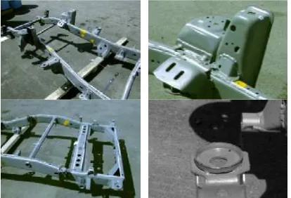
In this research we used VMS method for determining differences between reference chassis and produced one (figure1.) due to the quality assessment of product line and improving fixtures for making more accurate products. A none-metric digital camera and a proper network are used for collecting information from objects.
Professional EOS Digital SLR
Magnesium body, environmentally sealed, based on EOS-1V Integrated battery compartment /
vertical hand grip 11.4 megapixel CMOS sensor
(primary colour filter) Full frame sensor, no field of view
crop / focal length multiplier Output image size: 4064 x 2704 or
2032 x 1352
Table1. Camera properties. (Samadzadegan et al., 2004)
Figure 1. different components of the case study
2. MATHEMATICAL BACKGROUND
2.1 Network Design
In general, factors affecting the final accuracy of the object coordinate are shown in schema in Figure 2. Optimal level for each of the factors influencing the network design is obtained in it.
Figure2. Factors affecting accuracy of VMS systems.(GSI, 2000)
Important and necessary role of the network design and its implementation process to achieve the ultimate accuracy of the calculations is shown in figure (2).
VMS networks are substituted by their points. Determination of the network involves the determination of the coordinates of these points. Network qualification is linked to point coordinates (Atkinson, 1998). When we look for a correlation between the accuracy of the object coordinates and the accuracy of the image coordinates, we will find direct proportionality, but it is easy to see that there must be other factors, too. In accordance with the literature on close range photogrammetry (Fraser, 1996; Mason, 1995) the main factors are image scale, network redundancy and a design factor expressing the strength of the network. An initial precision indicator can be given by the equation (1) (Fraser, 1996):
a
Where c=experimental error of object coordinates X,Y,Z; S = scale of the image;
d = the object distance,
=average error of image coordinates; a=average error of angle measurement, q = design factor characteristic of the network,
k = ratio of independent perceptions and the number of images. For experimental close range photogrammetry design, the values of the factor qin equation (1) represents specific figures associated with each generic network of the network set, and they fall between 0.4 to 0.8 for favourable generic convergent multi-stage close range photogrammetric networks. The value k for a generic network is usually given as 1, and can be raised by adding more camera stations and/or multiple exposures, but the value can also be a fraction number depending on the correlation (Mason 1995).
2.2 Self-Calibration
The mathematical model of the self-calibrating bundle adjustment is based on the well-known collinearity condition which is implicit in the perspective transformation between image and object space:
(2)
The calibration terms in the equation (2) are represented by the principal point offsets x0, y0, the principal distance, c(interior orientation parameters) and the perturbation terms x and y which account for the departures from collinearity due to lens distortion and in-plane and out-of-plane focal plane distortion. The purpose of the present paper is to concentrate on the recovery of calibration parameters through the simultaneous solution of the collinearity equation (Slama, 1980).
In seeking appropriate parameters for the functions Ixand Iy, it is necessary to consider the four principal sources of departures from collinearity which are physical in nature. These are symmetric radial distortion, decentring distortion, image plane un-flatness and in-plane image distortion. The net image displacement at any point will amount to the cumulative influence of each of these perturbations (Brown, 1976). Thus,
(3)
Where the subscript r is for radial distortion, dfor decentring distortion effects, ufor out-of-plane un-flatness influences and f for in-plane image distortion. The relative magnitude of each of the images coordinate perturbations depends very much on the nature of the camera system being employed (Tarabanis, 1994 ).
2.3 Bundle adjustment
With adding the parameters discussed above, in bundle adjustment equations, given the high degree of freedom in convergent networks, the adjustment parameters will be calculated. The main advantage of this adjustment method is the
calculation of interior orientation parameters and object coordinates, in a free adjustment process (Mikhail, 1973).
(4) 1
2 0
, )
( + = =
=f x l v Ax C P
l l
Where, lis the observation vector image coordinates, vis the vector of random error, Ais the design matrix of equations, x is the vector of unknowns, Cl is the covariance matrix of
observation, 02is the variance factor and P is the weight matrix
of observations. Then unknowns can be calculated using equation (5) (Vanicek et al., 1986):
(5) Pl
A PA A
xˆ=( t ) 1 t
Then, covariance matrix of the predicted parameters will be obtained using equation (6)
1 2
0( )
= APA
Cx t (6)
It is necessary to note that for approximation of precision of
predicted parameters, the predicted value for 02 that calculated in adjustment process will be used in above equation.
3. EXPERIMENTS AND RESULTS
With implementing conditions discussed later, a proper strong photogrammetric network created and imaging performed on the objects. Figures (3,4) show three-dimensional network structure of the objects from different views.
(a)
(b)
Figure 3. Network structure created for original chassis from top view(a), and side view (b)
(a)
(b)
Figure 4. Network structure created for produced chassis from top view(a), and side view (b)
For achieving proper accuracy in calculations, each target point of the chassis in the body surface, should be observed in at least six different stations with appropriate geometry. Given the observations, we tried to read much more numbers of specific points from the beginning and end points of the scale bars. This will cause the equations to calculate position of these points with higher degree of freedom in adjustment process and produce much better results.
3.1 Pre-processing of observations
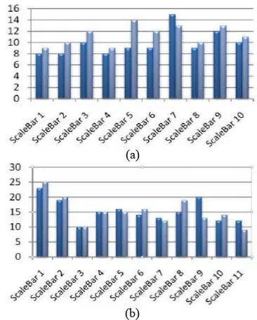
As described later, the quality of the results of calculations depend on several factors. The most important of them are the strength of the photogrammetric network geometry, number of observation redundancy and accuracy of the target points coordinates. For example, in the figures (5) the numbers of observations, performed for reading two points for scale bars from different stations are shown.
(a)
(b)
Figure 5. Numbers of observations for start and end of scale bars in main chassis (1) and produced one (2).
3.2 Adjustment and self-calibration results
After reading the points, bundle adjustment with self-calibration performed. In this section of calculation, initial values of interior orientation parameters entered in equations as the weighted values and then the precise value of them determined again. Among the other outputs of this section, are the coordinates of points and the exterior orientation parameters of the camera.
The values obtained for interior orientation parameters, achieved from observations in both main and produced chassis (Table 2). K2and K3are eliminated because of high level of correlation between them.
R
Table 2. Interior orientation parameters
3.3 Quality control of results
To ensure of achieving accurate results, it is required to perform statistical tests on the values of the adjustment process. In this study three tests performed for this aim.
a) Test of variance factor
At the beginning of adjustment, the initial value for variance
factor ( 02) has been set to 1. After performing adjustment,
estimated value for this quantity ( ˆ ) in two data sets achieved 02 as table (3). So, according to the high amount of degree of freedom, and avoiding observations from probable systematic errors, the test of variance factor performed for estimated variances in 95% confidence level (Vanicek et al., 1986). The test result accepted in related confidence level. It means that with 95% probability, there is not gross error in observations.
Product
Table 3. Adjustment properties
When ˆ02 achieved correctly, it is possible to calculate the accuracy of results as described later. Highest and lowest achieved accuracies of two chassis are shown in tables below.
Main Chassis X Y Z
Table 4. Accuracy of points considering RMSE in main chassis.
Table 5. Accuracy of points considering RMSE in produced chassis.
These results demonstrate the capability of this approach, because in the worst case, the achieved accuracy is better than 200 microns.
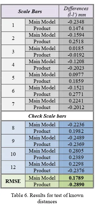
b) Test of network using known lengths
The method that can be done through the calculation of the network stability is investigated by measuring the lengths. To do this, the lengths of scale bar have been estimated from resulted coordinates again. To do so, some of scale bars will be entered in equations for obtaining scale amount and the others will be used as check value. So, it is possible to compare the resulted amount of scale bar with the correspondence lengths that measured directly on the object to obtain goodness of adjustment quality and internal accuracy.
Scale Bars Differences
(l-l') mm
1 Main Model -0.2348
Product 0.1474
2 Main Model -0.1594
Product 0.2518
3 Main Model 0.0185
Product -0.0192
4 Main Model -0.1208
Product -0.2023
5 Main Model 0.0977
Product 0.1859
6 Main Model -0.1521
Product 0.2771
7 Main Model 0.2241
Product -0.2012
Check Scale bars
8 Main Model -0.2236
Product 0.1982
9 Main Model -0.2489
Product -0.2369
10 Main Model 0.2805
Product 0.2389
12 Main Model 0.2298 Product -0.2376
RMSE Main Model 0.1789 Product -0.2890
Table 6. Results for test of known distances
As table (6) indicates, at this stage, five scale bars are selected to use as check value. With recent calculations, the amounts in differences, noted that the dispute was not unusual in the first and second stage results of calculations.
c) Considering correlations between parameters
Depending on the acceptable correlation between exterior and interior orientation parameters, it can be concluded that the network is suitable for observation (Grun 1980). As explained earlier, the correlation value between the parameter should be smaller than 0.7 (Fraser, 1996).
With respect to the values that demonstrated in figure (6), the largest correlation value in both series of results is 0.64, indicating the strength of designed network and observations.
3.4 Distortion Analysis in Chassis
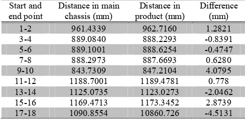
This section is a very important part of the calculation. The results of this section will help the manufacturer to improve products quality due to producing parts more similar to the main part. To this end, the output of computational steps that we mentioned earlier will be used in the input of distortion analysis. For this purpose, the distances between the interested points of both chassis will be measured in two X and Y directions. Then correspondent distances between two chassis are compared.
Start and end point
Distance in main chassis (mm)
3-4 889.0840 888.2293 -0.8391
5-6 889.1001 888.6254 -0.4747
7-8 888.2973 887.6693 0.6280
9-10 843.7309 847.2104 4.0795
11-12 1188.7001 1189.4781 0.778
13-14 1125.0735 1123.0273 -2.0462
15-16 1169.4713 1173.3452 2.8739
17-18 1090.8554 10860.726 -4.5131
Table 7. Final results for critical points on both chassis
It is necessary to obtain that, all of the points subjected to discussed comparison, are specific points have significant role in making fixtures. So, these differences will be used directly in improving fixtures size and positions.
4. CONCLUSION AND REMARKS
To achieve better levels of precision in the industry bodies such as the chassis, it is necessary to use retro reflective targets with imaging in specific conditions for detecting targets more suitable and with high level of precision. This method will reduce the time needed for observation too.
In this research we used some feature points and measured distance between them for introducing scale value with traditional precise tools. For avoid or reducing the error caused by measuring the lengths of the Scale-Bar, authors purpose to use standard scale bars. Furthermore, since the importance of strength of the photogrammetric network, it is proposed that the researchers to investigate network design as a problem of optimization, and use artificial intelligent solutions for creating more strong networks.
The results of this study indicate the high potential of Vision Metrology System for industrial applications. Given the obvious advantages of this method, it is recommended to implement of it for quality control and improvement of industrial assembly lines, especially in automotive production.
5. REFERENCES
Samdzadegan, F., Hahn, M., Mostofi, N., 2004. Geometric and Radiometric Evaluation of the Potential of a High Resolution CMOS-Camera.20th
International Congress for Photogrammetry and Remote Sensing, ISPRS, Istanbul, Turkey.
Atkinson, K.B., 1998. Close Range Photogrammetry and Machine Vision. Whittles Publishing, Scotland, 384 pages.
Fraser, C.S., 2001a. Automated off-line digital close-range photogrammetry: capabilities and applications. 3th International Image Sensing Seminar on New Developments in Digital Photogrammetry, GIFU, Japan, pages 22-30. 2
Ganci, G. and H. Handley (1989). Automation in
Videogrammetry. Real-Time Imaging and Dynamic Analysis, ISPRS, Commission V, Working Group V/1, Hakodate, Japan,.
Fraser, C.S., 1989. Precise alignment and verification by photogrammetry. Proceedings, 11th ESTEC Workshop on Antenna Measurements, ESA Publication WPP-001, Gothenburg, pages 109-114.
GSI, 2000. Manual of V-STARS: a vision metrology system. Geodetic Services Institute, 60 pages.
Fraser, C.S., 1996. Network design. In K.B. Atkinson, editor, Close Range Photogrammetry and Machine Vision. Whittles Publishing, Roseleigh House, Latheronwheel, Caithness, KW5 6DW, Scotland, UK, Chapter 9, pages 256-281.
Mason, S. (1995). Expert System-Based Design of Close Range Photogrammetric Networks. ISPRS Journal of Photogrammetry and Remote Sensing 50(5): 13-24.
Slama, C.C., 1980. Manual of Photogrammetry. Fourth Edition. American Society of Photogrammetry and Remote Sensing, Falls Church, Virginia, USA.
Brown, D.C., 1976. The bundle adjustment û progress and prospects. International Archive of Photogrammetry, Paper No. 3-30, 33 pages.
Tarabanis, K., Tsai, R.Y., Allen, P.K., 1994b. Analytical characterization of the feature detectability constraints of resolution, focus, and field-of-view for vision sensor planning. Computer Vision, Graphics and Image Processing: Image Understanding, 59(3):340-358.
Mikhail, E.M., 1973. Recursive methods in photogrammetric data reduction. Photogrammetric Engineering, 39(9): 983-989.
Vanicek, P., Krakiwsky, E., 1986, Geodesy: The concepts. North Holland, Amsterdam (2nd Edition).
Grun, A., 1980. Precision and reliability aspects in close range photogrammetry. International Archive of Photogrammetry, 23(B11): 378-391.
1
Figure 6. Correlation of parameters, main part (a), product(b)