Unit root tests in the presence of uncertainty
about the non-stochastic trend
Leila Ayat, Peter Burridge
*
Department of Economics, University of Birmingham, Edgbaston, Birmingham B15 2TT, UK
Received 1 November 1996; received in revised form 1 December 1998; accepted 1 April 1999
Abstract
A sequential procedure for determination of trend degree and testing for a unit root is introduced; its properties are investigated by Monte Carlo experiment. We implement the pseudo-GLS unit root tests of Elliott et al. (1996. Econometrica 64(4), 813}836), with lag length selected by the BIC criterion. Our procedure allows for quadratic trend, and we introduce a&GLS'-type test for this case. We compare the sequential procedure, in which trend degree is tested after a unit root pre-test, with a robust trend test recently developed by Vogelsang (1998. Econometrica 66(1), 123}149). The sequential procedure is advocated in preference both to informal use of the usual family of unit root tests and to alternative formal sequential methods that have been advanced in the literature. It is illustrated by application to the inventory data analysed in Hall (1994. Journal of Business and Economic Statistics 12(4), 461}470). ( 2000 Elsevier Science S.A. All rights reserved.
JEL classixcation: C22
Keywords: Unit root tests; Trend degree; Sequential strategies
1. Introduction
In practice, testing for a unit root takes place in the presence of uncertainty about the appropriate degree of any deterministic trend that the data may
*Corresponding author. Tel.:#44-121-414-6640; fax:#44-121-414-7377. E-mail address:[email protected] (P. Burridge)
contain. Consequently, unit root tests are often conducted after some kind of pre-test for the trend; such pre-tests may be very informal, such as inspection of
time plots of the data, or may be implemented by testing the signi"cance of the
coe$cient on the time trend in an equation "tted to the data. Whether such
pre-tests are employed or not, it is very common for the various test statistics not to agree, as reported, for example, by Hall (1994) who applied the ADF
qkandqqtests (see below) to 10 inventory series,"nding that the tests were in
agreement in roughly half the series.1Commenting on the disagreements, Hall
(1994, pp. 467}468) observes,
Clearly there can be disagreement between the results of the tests due to the
inherentvariation in sampling. There are two alternative explanations that
need to be considered,however. First,ifqkis insignixcant butqqis signixcant,
then it may be due to misspecixcation of the trend term.West(1987)
demon-strated that ify
tis stationary about a linear time trend but the trend is omitted
from the regression model, thenqkconverges in probability to0,so
asymp-totically one never rejects a unit root. Therefore I interpret this type of
conyicting result as evidence against a unit root. Similarly,ifqkis signixcant
butqqis insignixcant,then this may be due to the inclusion of a redundant
regressor. Dickey (1984) demonstrated that if y
t is stationary about an
intercept alone, then the inclusion of a linear time trend2leads to a
con-siderable loss of power. Therefore I also interpret this type of conyict between
the tests as evidence against a unit root.
The interpretive issue raised in the above comment arises in all applications of unit root tests, and the procedure we propose is designed to provide a systematic
resolution of the problem via evaluation of the signi"cance of the trend.2This
idea is not completely new, of course; the "rst proposal for a sequential
procedure we can "nd appears in Perron (1988), and Dolado et al. (1990)
advocated the sequential use of the Dickey}Fuller unit root tests and tests for
the presence of a trend. So far as we are aware, however, there has been no subsequent study of the properties of such sequential tests, in spite of the no doubt very wide use of informal strategies of this type in empirical work. Given
the attention devoted in the literature to modifying Dickey}Fuller tests (and
their variants) in order to control test size, the failure to examine the properties of the sequential decision rules within which they are generally employed is
a serious omission. The present paper begins to"ll this gap.
In some settings, such as the estimation of average growth rates, the non-stochastic trend function may itself be the focus of interest, and we might hope to
1Hall's study compares lag length selection via information criteria, with selection by general to speci"c and speci"c to general testing, and he"nds that unit root test outcomes are in some cases sensitive to the method used. See Section 5 for further discussion.
be able to draw inferences about the trend which are robust to the autocorrela-tion structure of the stochastic component. Vogelsang (1998) develops test statistics with size which is controllable irrespective of the stationarity or non-stationarity of the shocks, while Canjels and Watson (1997) explore the
e$ciency of various trend estimators in the same setting. While these latter
papers focus on the construction of con"dence intervals for trend estimates, we
are primarily concerned with determining trend degree, so that size and power are both important.
Section 2 sets out the data-generation process assumed, and de"nes the unit
root tests used. The sequential procedures are de"ned in Section 3. These
procedures could be implemented using any of the many forms of unit root test statistics that are now available, but in view of their good power, we illustrate
their performance using the&GLS'forms of the ADF test introduced by Elliott et
al. (1996) extended here to allow for a quadratic polynomial trend. Trend degree
is tested either by conventional t-tests (with their standard critical values)
applied to levels or to di!erences of the data depending on the outcome of a unit
root pre-test, or using a robust test due to Vogelsang (1998) for which no pre-test is required. The quadratic trend is included as a default class: if the tests detect
such a trend, then the series should not be modelled with a linear trend alone.3
A feature of the fully sequential procedure we study is that tests for the degree
of the trend are conducted after a unit root pre-test, with the highest trend
degree maintained, has been used to determine whether or not to di!erence the
data. This is only one possibility, however; in Section 3 we reject on grounds of
redundancy the use of joint F-type tests for unit roots and trend, and in the
Monte Carlo experiment described in Section 4 we illustrate the e!ect of
replacing the&t'tests for trend degree with a robust test. Section 5 applies the
procedures to the inventory data studied by Hall (1994), and concludes.
2. Data-generation process,test de5nitions and invariance properties
2.1. The DGP
We write the data, y
t, as the sum of a deterministic (polynomial trend)
component,d
t, and a purely stochastic component,ut:
y
The model selection and hypothesis testing problem is to determine the degree
of d
t, and to test o"1, against trend-stationary alternatives, DoD(1. In the
leading case,v
tis IID(0, p2); departures from this may be handled in a variety of
ways, but following Hall (1994), we have used the ADF approach with lag length selected via an information criterion, as this is simple to implement and
per-forms well in most cases}see Stock (1994) for a recent survey. Whatever method
of individual test size-correction is employed, the contribution to overall size from the sequential procedure is likely to be similar, and this is our main
concern. The initial observation is treated as random, and thus lies o!the trend,
in general.
2.2. The Dickey}Fuller family of unit root tests
The currently most widely employed tests for a unit root, the so-called &augmented'versions of those developed by Dickey and Fuller (1979, 1981), are
based on the t-statistic foro"1 in the OLS regressions:
*y
To these widely used tests we may add the test introduced by Ouliaris et al. (1989), based on
The test equations, being augmented withplags of*y
ton the right-hand side,
thus approximatev
t by a stationary AR(p). There are a number of equivalent
ways of calculating the test regressions; for ease of comparison with the&GLS'
tests discussed below and implemented in our experiments, we can think of
partitioning the regression into a "rst stage removal of the trend by OLS,
followed by OLS estimation of (2a) applied to the detrended series (augmented
The DF}GLS tests of Elliott et al. (1996) (ERS), di!er from (2b)}(2d) in that the trend is estimated by pseudo-generalised least squares. The GLS test statistics are thus de"ned as the&t'statistic on the coe$cient ofyH
t(no detrending, corresponding to (2a)), or
yH
t"yt!bK00,GLS (4)
(de-meaned only, corresponding to (2b)), or
yH
t"yt!bK01,GLS!bK11,GLSt (5)
(de-meaned and de-trended, corresponding to (2c)), or
yHt"y
t!bK02,GLS!bK12,GLSt!bK22,GLSt2 (6)
(de-meaned and quadratic de-trended, corresponding to (2d)).
The&GLS'regressions di!er in the three cases, since in each case the
quasi-di!erencing operator is chosen by setting the test asymptotic power function
(against a sequence of alternatives,o"1#c/¹) tangent to its power envelope
at a power of 50% when size is set at 5%. ERS obtainedc60"!7.0 (de-meaned)
and c61"!13.5 (de-meaned and de-trended), but did not investigate higher degree tests.
To obtainc6 for the quadratic trend test we followed ERS and set size at 5%,
and sought that value ofc6 which would yield asymptotic power of 50%. To do
this, we took¹"1000 and estimated the power at variouscvalues using 20,000
Monte Carlo replications. The value ofc6 obtained was!18.5; we then checked
the power for this value ofcat¹"500 (i.e.o"0.963) and found it to be very
close to 50%, thus con"rming thatc6
2"!18.5 is appropriate, since the power
is unchanging as¹increases from 500 to 1000. Critical values for this new test
are given in Appendix B.
Writing o6
j"1#c6j/¹, (j"0, 1, 2) we can de"ne the bKij,GLS as follows. bK00,GLSis the OLS regression coe$cient obtained by regressing the vector,
[y
on the vector,
[1, 1!o6
0,2,1!o60]@,
similarly, [bK01, bK11]@
GLSresults from the OLS regression of the vector,
[y
GLSresults from the OLS regression of the vector,
[y
ERS "nd that in practical sample sizes, the GLS-detrended unit root tests enjoy a power advantage over their OLS-detrended counterparts. The
asymptotic e$ciency gain in trend estimation is substantial when the data are
near-integrated, and has been quanti"ed by Lee and Phillips (1994). In "nite
samples, the e$ciency of the trend estimates may be calculated exactly when
v
tin (1) is a stationary ARMA process, and the pseudo-GLS trend estimates are
not, in general, more e$cient than OLS (see Canjels and Watson, 1997);
however, the power advantage of the ERS tests remains because the null distribution of the tests is shifted to the right relative to the corresponding
Dickey}Fuller distributions (some evidence on this point is contained in
Burridge and Taylor, 1999).
As is well known, the three regressions (2a)}(2c) give unit root test statistics,
q,qkandqq, respectively, with di!erent invariance properties and limit
3. Sequential testing strategies
Since we are assuming that the degree of any polynomial trend that may be present in the data is unknown, the objective of the testing strategy should be to
identify the class of model, that is, to test the unit rootanddetermine the trend
degree. To this end we consider a sequence of pre-tests.
If the data are generated by (1), witho"o
0, known,vt&IID(0,p2), but the
trend parameters unknown, then"tting equation (2b), (2c), or (2d) without using
our knowledge of o produces ine$cient trend estimates in "nite samples;
e$cient estimation, by GLS, requires the dependent variable to be transformed
to (1!o¸)y
t"yst, say.4Ifo"1 this leads to yst"*y
t"(b1!b2)#2b2t#vt (7)
ifk"2, or
yst"*y
t"b1#vt (8)
if k"1; in either case, the non-stochastic component may be e$ciently
esti-mated and its signi"cance tested by standardt-tests. Furthermore, as shown by
Dickey (1984) and West (1987), unit root tests lose power if the trend speci"ed is
of higher degree than necessary (via ine$cient estimation ofo), and are
incon-sistent (biased in favour of the null) if the trend"tted is of lower degree than is
present in the DGP. To minimise such power losses, we seek reliable inference
about the trend in the presence of uncertainty about o. At the same time, we
want reliable inference aboutoin the presence of uncertainty about the trend.
The invariance results set out in Appendix A combined with more e$cient trend
estimation using (7) or (8) if unit root pretests applied to (2d) or (2c) fail to reject, suggest a strategy which we now describe in detail.
The most general maintained model allows for a quadratic trend:
y
t"b0#b1t#b2t2#ut. (9)
With (9) maintained, we can obtain a unit root test statistic invariant tobfrom
regression, (2d) or the &GLS' variant, and this test forms the "rst step of our
sequence. At every step of the sequence the lag order,p, must be chosen; in our
experiments, this was done by minimising the Schwarz information criterion
(BIC), ln(p(2)#p.ln(¹)/¹, with 3)p)8 (the lower bound being used for
4As pointed out by a referee, the OLS trend estimates in regressions (7) and (8) are asymptotically equivalent to GLS even ifv
comparability with the results of ERS, who impose this). We comment further on this after setting out the procedure; the complete algorithm is:
3.1. Strategy S1
1. Perform a preliminary unit root test invariant to quadratic trend under the null.
2(a). If the unit root is not rejected at step 1, provisionally maintain this
hypothesis and estimate *y
t"bH01#bH11t#+pj/1aj*yt~j#et, testing for the
null that k"1, (that is, b2"0, in (9)) using thet-statistic on bH11 referred to standard tables.
2(b). If the unit root isrejectedat step 1, test fork"1 using thet-statistic on a(
223(a). Ifin Eq. (2d), again referred to standard tables.k"1 was rejected at step 2, we stop, since the unit root test already
conducted is the only one available which is invariant to the maintained quadratic trend.
3(b). If k"1 was not rejected, and the unit root was not rejected, perform
a second provisional unit root test invariant to linear trend under the null.
3(c). Ifk"1 was not rejected, but the unit rootwasrejected at step 2, test for
k"0 using thet-statistic ona(
11in (2c) referred to standard tables and stop.
4. If the unit root was not rejected at 3(b), estimate *y
t"
bH00#+pj
/1aj*yt~j#et, testing the null thatk"0 using thet-statistic onbH00.
5(a). Ifk"0 is rejected at step 4, stop.
5(b). Ifk"0 is accepted at step 4, conduct a further provisional unit root test
invariant to the mean under the null.
6(a). If the unit root is not rejected at 5(b), test the magnitude of the initial
observation,y
1, relative to the increments inyusingy1/JM¹~1R(*yt)2Nreferred
to N(0, 1).
6(b). If the unit root is rejected at 5(b), stop. 7(a). Ify
1di!ers signi"cantly from zero, stop.
7(b). Ify
1does not di!er signi"cantly from zero, perform a unit root test which
is not invariant to the mean under the null.
In many applications, steps 1 and 2, and steps 6 and 7, will be redundant, so we have also simulated a shorter sequential strategy:
3.2. Strategy S2
Start from step 3(b),"nish at step 5.
3.3. Strategy S3
Test for the presence of linear trend using Vogelsang's (1998)t-PS1 statistic. If
no trend is detected, perform a unit root test invariant to the mean under the
null; if trendisdetected, perform a unit root test invariant to linear trend under
the null.
3.4. Strategy S3*
Test for linear trend using botht-PS1 and the standardt-statistic normalised
by¹~1@2(referred to critical values in Table II(ii) of Vogelsang, 1998), rejecting
the no-trend null if either test rejects and proceeding as in S3.
Before commenting on other possible sequences of tests, we make some general observations.
(a) Our treatment of the trend and extra lags presupposes that not more than
one unit root may be present, as we now illustrate for the case,p"1. Suppose
u
tis the non-stationary AR(2):
*u
t"/*ut~1#et, (10)
whiley
tis given by Eq. (9), withb2possibly zero, to be tested. Assume for the
moment thatpis known. The"rst stage unit root test will be based on estimates
from the equation
y
t"oyt~1#t*yt~1#a02#a12t#a22t2#error, (11)
while the DGP implies that
*y
t"(b1!b2)#2b2t#/*ut~1#et. (12)
Substituting for*u
t~1using (9) and rearranging, we"nd
y
t"yt~1#t*yt~1#Mb1(1!t)#b2(3t!1)N#2b2(1!t).t#et.
(13)
If the unit root test using (11) fails to reject the null, our procedure, S1, then tests
the coe$cient ontin (14) estimated in di!erences
*y
t"t*yt~1#Mb1(1!t)#b2(3t!1)N#2b2(1!t).t#et (14)
which is e$cient providedtO1, that is, provided there is only a single unit root
inu
(b) Choosing lag length via the BIC criterion applied at each step produced the same results in our experiments as choosing lag length only at the odd-numbered steps and retaining this length, but we cannot rule out the possibility that the former could be advantageous in some situations, and so that is what we recommend.
The S1 algorithm has eight possible outcomes: (i) quadratic trend#unit root,
(ii) quadratic trend#stationary, (iii) linear trend#unit root, (iv) linear
trend#stationary, (v) non-zero mean#unit root, (vi) non-zero mean#
stationary, (vii) zero mean#unit root, (viii) zero mean#stationary. The
process chosen is the same for outcomes (v) and (vii) (unit root, no trend), and also for (vi) and (viii) (stationary, no trend). For a pure unit root test, the size (or power) of the algorithm is thus the sum of the proportions of even outcomes,
while the probability that a linear trend is identi"ed is the sum of the
propor-tions in outcomes (iii) and (iv), and so on. In reporting the experimental results in the next section we concentrate on three issues: overall size/power for
the null,o"1; size/power for linear trend; proportion of correct model
identi-"cations.
A feature of the S1 and S2 algorithms is that non-rejection of a unit root at an earlier step can be overturned later if the data allow trend degree to be
re-duced, but not vice-versa.5 This accords with what most researchers would
do in practice. As sample size increases, the overall size of the unit root test in the sequential algorithms will reduce in the presence of a linear trend be-cause of the power of the trend degree tests. The non-zero size of the latter will
result in the trend in some series being misclassi"ed as of too high degree,
however.
The behaviour of the S1 and S2 algorithms re#ects the interplay between test
power at any given step and the quality of the approximation to the sampling
distribution of thet-statistic delivered at the succeeding step. For example, in S1,
if the preliminary unit root test has low power (as whenois moderately large),
then trend stationary series will often go to Step 2A, in which the degree of the
trend is tested in a misspeci"ed equation. This has the e!ect of reducing the
probability that a stationary process with a linear trend is correctly identi"ed if
it also has a large AR root. Similarly, in situations in which unit root tests
remain over-sized even after augmentation by lagged di!erences, trend degree
will be tested by applying thet-statistic to inappropriate critical values. In fact,
as shown by our Monte Carlo experiments, such e!ects do not appear to
seriously undermine the performance of the S2 procedure, when compared with
use of Vogelsang's robust trend test in S3.
3.5. Alternative sequential procedures
Perron (1988, pp. 316}317) proposes a strategy (in each case using the
Phillips}Perron modi"ed DF tests) which seems to amount to the following.
Estimate Eq. (2c) and test
H
01: [(o#!1),a0#, a1#]"[0, a0, 0],
using theF-test,U
3, of Dickey and Fuller (1981). If this null is not rejected, test
H
02: (o#!1)"0
with the unit root test, and if the null is rejected here, stop. If neither H
01nor
2. If H03is rejected, stop. Otherwise, estimate Eq. (2b) and test
H
04: [(o"!1),a0"]"[0, 0],
using theF-test,U
1. If this null is not rejected, test
H
05: (o"!1)"0,
using the unit root test, and if the null is rejected here, stop. If neither H
04nor
H
05is rejected and the series has a zero mean then test
H
06: (o!!1)"0.
As with our strategy, the aim is to use the unit root test with most power;
however, the outcomes of the threeF-tests may be ambiguous: whatshouldwe
do if, say, H
03is rejected and H02is not?. In Perron's strategy we implicitly treat
rejection of H
03as evidence of the presence of drift, not as evidence against the
unit root, which clearly it could be. It seems to us that these jointF-tests will
generally beg the question of whether it is the unit root or non-stochastic part of
the null which is to be rejected; to interpret theU-type tests, therefore, one would
need to conduct a separate test for trend degree. The S1}S3 procedures do this.
A much simpler decision rule that has been advocated, according to folklore, (we have not found it in print) is
Test H
06, and if the test rejects, stop.
Test H
Size/power of sequential rules, all tests nominal level 5%
S1"Allow quadratic trend and use&t'tests For each DGP, C1"Size/power againsto(1
S2"Allow linear trend and use&t'tests C2"Size/power against TrendO0
S3"Allow linear trend and use Vogelsang tests C3"Proportion correct model identi"ed
S1 0.71 0.73 0.65 0.57 0.57 0.50 0.74 0.85 0.66 0.97 1.0 0.93 0.86 0.95 0.78 0.70 0.70 0.63 0.72 0.72 0.61 S2 0.68 0.70 0.68 0.54 0.53 0.53 0.70 0.83 0.70 0.93 1.0 0.93 0.82 0.94 0.82 0.66 0.67 0.66 0.66 0.66 0.66 S3 0.67 0.93 0.67 0.37 0.45 0.36 0.70 1.0 0.70 0.93 1.0 0.93 0.82 1.0 0.82 0.58 0.73 0.58 0.51 0.62 0.50 Trend"0.2Ht 1.0
S1 0.08 0.51 0.39 0.09 0.26 0.13 0.06 0.80 0.69 0.65 1.0 0.34 0.12 0.95 0.80 0.11 0.32 0.18 0.16 0.31 0.13 S2 0.05 0.47 0.42 0.07 0.18 0.14 0.04 0.79 0.75 0.53 1.0 0.47 0.08 0.95 0.87 0.07 0.25 0.20 0.10 0.21 0.15 S3 0.04 0.13 0.10 0.04 0.04 0.02 0.04 0.31 0.27 0.53 1.0 0.47 0.07 0.54 0.46 0.05 0.07 0.04 0.07 0.06 0.03 0.95
S1 0.11 0.53 0.08 0.12 0.18 0.07 0.12 0.95 0.09 0.76 1.0 0.58 0.18 1.0 0.13 0.14 0.26 0.09 0.20 0.26 0.12 S2 0.08 0.51 0.08 0.09 0.13 0.07 0.09 0.94 0.09 0.66 1.0 0.66 0.13 1.0 0.13 0.10 0.20 0.10 0.14 0.19 0.13 S3 0.08 0.25 0.08 0.05 0.06 0.03 0.09 0.51 0.09 0.66 1.0 0.66 0.13 0.74 0.13 0.07 0.12 0.06 0.07 0.10 0.06 0.90
S1 0.21 0.67 0.18 0.19 0.24 0.15 0.20 0.98 0.16 0.86 1.0 0.73 0.33 1.0 0.27 0.25 0.34 0.20 0.31 0.36 0.24 S2 0.18 0.65 0.18 0.16 0.20 0.15 0.17 0.98 0.17 0.80 1.0 0.80 0.28 1.0 0.28 0.21 0.30 0.21 0.25 0.30 0.24 S3 0.17 0.47 0.18 0.08 0.14 0.08 0.17 0.78 0.17 0.80 1.0 0.80 0.28 0.94 0.28 0.15 0.26 0.15 0.14 0.22 0.14 0.70
S1 0.71 0.99 0.65 0.57 0.66 0.51 0.74 1.0 0.66 0.97 1.0 0.93 0.86 1.0 0.78 0.70 0.84 0.63 0.72 0.82 0.62 S2 0.68 0.99 0.68 0.54 0.64 0.54 0.70 1.0 0.70 0.93 1.0 0.93 0.82 1.0 0.82 0.66 0.82 0.66 0.66 0.78 0.66 S3 0.68 0.99 0.68 0.50 0.75 0.50 0.70 1.0 0.70 0.93 1.0 0.93 0.82 1.0 0.82 0.66 0.93 0.66 0.64 0.88 0.64
L.
Ayat,
P.
Burridge
/
Journal
of
Econometrics
95
(2000)
71
}
96
Test H
02, and if the test rejects, stop. Testo"1using(2d).
(The"nal step being added by us.)
This rule has been justi"ed informally on the grounds that the"rst two tests are under-sized and lose power when an intercept or non-stochastic trend are
present. However, the rule is not truly sequential, since it is equivalent to&reject
the unit root when at least one of the tests rejects'. Viewed solely as a unit root test
(as it must be), this procedure has slightly greater size and power than S1, but leaves the trend degree uncertain.
4. Experimental results
Table 1 reports the results of 5000 replications of S1}S3 using the ERS
&GLS'-type ADF tests in the following design:
(a) sample size,¹"100, all series initialised at zero att"!25, so that when
DoD(1, the sample fromy
(e) nominal size of 5% for all tests
4.1. Behaviour under the unit root null
S1}S3 have di!erent overall signi"cance levels (against the null thato"1),
re#ecting the di!erent numbers of unit root tests performed. With no trend, and
when the serial correlation correction works e!ectively (for IID or AR(1)
shocks), S1 has actual size about 11%, S2 has size about 8%, and S3 size about 7%. Since only one unit root test is performed in S3, one might expect the size to be no greater than 5%; however, the data-dependent lag selection employed,
together with the use of approximate critical values for the ERSqk
GLStest (i.e.
those for theDFqtest}see ERS, 1996 for details) results in some size in#ation
even for IID shocks. Vogelsang's trend test is, except for the positive MA root
case, better sized than the unit-root pre-test based&t'test used in S2, while the
unit-root pre-test-basedt-test for quadratic trend used in S1 is also over-sized
(compare C2 in the"rst two rows of Table 1). We thus"nd that in the absence of
a trend, S3 identi"es the correct model more often under the unit-root null than
S1 or S2.
With a small trend (0.1t, equal top2e/10 per period), the unit root test sizes of
test used in S3 now reverses the ranking on C3, the proportion of correct model
identi"cations. Only when the presence of a positive MA or negative AR root
in#ates the trend test power do any of the algorithms correctly identify the
random walk with drift in more than one sample in four. When the trend
increases to p2e/5 per period, S2 is a clear winner because S1 too frequently
identi"es a spurious quadratic trend, while the S3 trend test still lacks power.
4.2. Behaviour under the(trend)stationary alternative
Except when there is a large MA root, the probability of correct model
identi"cation, C3, is U-shaped as o varies from 1 to 0.70, re#ecting the low
power of unit root tests for alternatives close to the null. When no trend is present, S1 is the most successful algorithm, measured by C3, for all stationary alternatives, because the extra power against the unit root outweighs the
probability of "nding a spurious quadratic trend. We may, however, not be
indi!erent between the various types of errors that go to make up (1!C3),
the probability of an incorrect model identi"cation.
When the trend is small, S2 is always better than S1, and always as good as S3, and better in the case of positive AR or negative MA roots. For the larger trend,
the ranking is the same, although the di!erences are smaller.
Following a referee's suggestion, we investigated the use of the normalised
t-statistic,¹~1@2t!=
Tin Vogelsang's terminology, to test for the trend in S3H.
The idea here is that in stationary series this test will be very conservative, contributing neither to size nor to power, but that it has better power under the
unit root null than does t-PS1. The results, not tabulated, show that for
o)0.95, adding this test to S3 makes no di!erence except when trend"0.2t; in
the latter case, power to detect trend is increased, but never exceeds that of S2. Wheno"1, we"nd slight size-in#ation of the trend test except whenh"0.5 or 0.8, so that for zero trend, S3 is better than S3H, while if trend"0.1tor 0.2t, S3H
is e!ectively the same as S2.
4.3. Some general comments
We have reported results with the nominal size of every individual test held at 5%, which produces algorithms with actual size (against the unit root null) greater than this, even when the shocks are serially uncorrelated. Results for nominal size 1 and 10% were also produced, but have been omitted to save
space}the patterns revealed were similar}the main notable feature being that
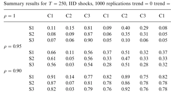
Table 2
Summary results for¹"250, IID shocks, 1000 replications trend"0 trend"0.1ttrend"0.2t
o"1 C1 C2 C3 C1 C2 C3 C1 C2 C3
S1 0.11 0.15 0.81 0.09 0.40 0.29 0.08 0.87 0.75 S2 0.08 0.09 0.87 0.06 0.35 0.31 0.05 0.85 0.80 S3 0.07 0.06 0.90 0.05 0.10 0.06 0.05 0.18 0.14
o"0.95
S1 0.66 0.11 0.56 0.37 0.51 0.32 0.37 1.0 0.32 S2 0.61 0.05 0.56 0.33 0.47 0.33 0.33 1.0 0.33 S3 0.56 0.03 0.54 0.28 0.51 0.28 0.32 0.71 0.32
o"0.90
S1 0.91 0.14 0.77 0.82 0.89 0.75 0.82 1.0 0.75 S2 0.87 0.07 0.81 0.78 0.86 0.78 0.78 1.0 0.78 S3 0.82 0.03 0.79 0.76 0.92 0.76 0.78 0.98 0.78
o"0.70
S1 1.0 0.11 0.89 1.0 1.0 0.93 1.0 1.0 0.93
S2 1.0 0.05 0.95 1.0 1.0 1.0 1.0 1.0 1.0
S3 0.96 0.03 0.93 1.0 1.0 1.0 1.0 1.0 1.0
thought to be a priority. In this particular setting, there seems, on balance, to be no advantage in using the robust trend test to choose the unit root test, primarily because of its low power. However, this conclusion rests on the assumption that all modelling errors are equally costly. In a setting in which spurious trend detection in the presence of a unit root was particularly to be avoided, the S3 algorithm might be preferred, but not otherwise.
The experiments were repeated with a sample size of 250; results for IID shocks are given in Table 2, which provide further support for use of the S2 algorithm in this setting. Only under the unit root null, with no trend present does S3 do better.
5. Application to inventory series and conclusion
5.1. Inventory series
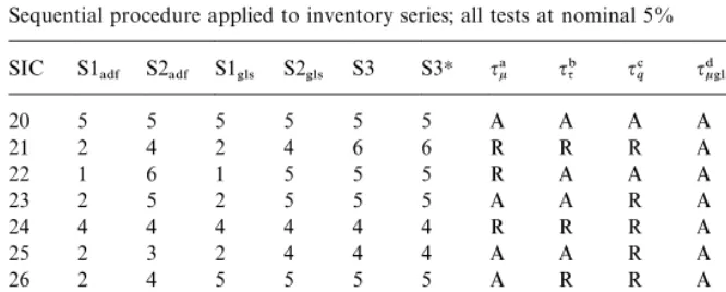
Table 3 reports the model classes identi"ed by the S1}S3 procedures, together
with the individual unit root test outcomes for the 10 US SIC inventory series studied by Hall (1994).
The data are monthly, seasonally adjusted, real dollar inventory holdings
running from 1958:12 to 1988:4.6Six versions of the sequential procedure are
Table 3
Sequential procedure applied to inventory series; all tests at nominal 5% SIC S1
!$& S2!$& S1'-4 S2'-4 S3 S3H q!k qq" q#q q$k'-4 q%q'-4 q&q'-4
20 5 5 5 5 5 5 A A A A A A
21 2 4 2 4 6 6 R R R A R R
22 1 6 1 5 5 5 R A A A A A
23 2 5 2 5 5 5 A A R A A R
24 4 4 4 4 4 4 R R R A R R
25 2 3 2 4 4 4 A A R A R R
26 2 4 5 5 5 5 A R R A A A
27 3 3 3 3 5 3 A A A A A A
28 1 3 1 3 3 3 R A A A A A
29 4H 4 4 4 4 4 R R R A R R
HNote: a,b,c,d,e,findividual test outcomes,R"reject. Key to cols2}7:
1"Quadratic trend#unit root. 2"Quadratic trend#stationary. 3"Linear trend#unit root. 4"Linear trend#stationary. 5"No trend#unit root. 6"No trend#stationary.
reported: ADF test-based, or GLS test-based, in each case with (S1) and with-out (S2) the quadratic trend tests, and the GLS test-based variants of
S3 and S3H. We used nominal size of 5% for every test, and a maximum lag
of 8.7
Note, "rstly, that there is substantial agreement between the ADF and the
GLS versions of the procedure: with the quadratic trend tests included, the only
disagreement is for SIC 26, which the ADF classi"es as stationary around
a quadratic trend and the GLS as having no trend but a unit root; without the quadratic trend tests there are three disagreements, SIC 22 being either trendless and stationary (ADF) or trendless and non-stationary (GLS), SIC 25 being either non-stationary around a linear trend (ADF) or stationary around a linear trend (GLS), and SIC 26 being either stationary around a linear trend (ADF) or non-stationary and trendless (GLS). In each of the latter three cases at least
one procedure identi"es a quadratic trend when this is tested for, suggesting that
the inferences based on a maintained linear trend may be fragile. Faced with the choice of GLS or ADF based inference, we would opt for the GLS tests here because of their greater power. It is notable also that the quadratic trend tests
reject the linear trend null for half the series: this is quite strong evidence against reliance on theqqtest result for these series; for example, SIC 23 is classi"ed as stationary around a quadratic trend if our full procedure is used, but as non-stationary and trendless otherwise.
Strategy S3 gives the same model as S2, except on SICs 21 and 27 in which no
trend is detected, while S3Hdetects the trend in SIC 27 but not in SIC 21. These
results using robust trend tests are thus remarkably consistent with those we obtain via sequential pre-testing.
A second important feature of the results is that the various unit root tests, taken individually, do not always agree. Focusing on the GLS tests, we see in Table 3 that all three tests (at nominal 5%) agree in only half the series. For the
series on whichqq'-4rejects a unit root, however, so also does the quadratic trend
test, and each of these series is classi"ed as stationary around a trend, an
outcome which echoes Hall's interpretation of the disagreements betweenqkand
qqwhich he found.
6. Conclusion
A sequential procedure for unit root testing and trend estimation has
been explored which has a clear advantage (simultaneous identi"cation of
trend degree) over a naive strategy which rejects a unit root when at least one of the DF family of tests rejects. Overall size of the procedure can be reduced by conducting each component test at a smaller size than is required. The ability of the procedure to correctly classify series with and without linear trends is dependent on the magnitude of the trend, and on the auto-regressive root, deterministic trends being much easier to detect when sto-chastic trends are absent. By using unit root tests as pre-tests before testing
trend degree (in a levels equation if the pre-test rejects, in a di!erenced
equation otherwise) we are able to avoid the use of the non-standard
sampl-ing distributions of the t-statistics on the trend coe$cients which arise
when the unit root is estimated in the equation used to test the trend. The size distortions which result are not negligible, but neither are they disastrous, measured by the probability of identifying the correct model (C3 in Tables 1 and 2).
The accommodation of level shifts and trend breaks into unit root testing procedures has been the subject of a number of recent studies, and is discussed at length by Stock (1994). We have not sought to incorporate these develop-ments into the strategy we propose, but extensions along these lines should be possible. The present study develops and illustrates a feasible model selection
strategy incorporating tests for both trend degree and unit roots, which clari"es
Acknowledgements
We thank Alastair Hall (who also supplied the inventory data), James Mac-Kinnon, John Nankervis, and other participants at the July 1996 ESRC Econo-metric Study Group meeting in Bristol, and two anonymous referees, whose comments have greatly improved the paper. All computations were performed in GAUSS. This research was supported by UK ESRC awards R00023 4797 and 6390.
Appendix A
We"rst present some convenient notation; as in the body of the paper, we writeo6
00GLS is the OLS regression coe$cient obtained by regressing the vector,
H
0y, on the vector, H0D0, while [bK01GLS, bK11GLS]@ results from the OLS
regression of the vector,H
1yon the matrix,H1D1, and"nally, [bK02GLS,bK12GLS,
bK22GLS]@ results from the OLS regression of the vector, H
2y on the matrix,
H 2D2.
A.1. Invariance results
We present the relevant results (for the case in whichv
tis IID) in Proposition
1, extension to the AR(p) case being covered in a remark.
Letu"[u
2,2,uT]@, u0"[u1,2,uT~1]@. Suppose the non-stochastic trend is
of degree,k, with coe$cients,b(k)"[b0,2,bk]@, and introducec(k), the vector of
coe$cients,ci, which solve the equation,
We may now write the DGP as
y"D
kb(k)#u, (A.2)
withy
0"Dkc(k)#u0, andu"u0o0#v,v&N(0,p2I).
Proposition 1. If the DGP is(A.2),and the equationxtted to the data is
y"[D
(b) If (A.3) is estimated by xrst detrending y and y
0 by pseudo-GLS and then
estimatingyH"yH0o(#e,by OLS,the&t'statistic for testingo"o
where the distribution of the randomvector,
w(k)"[[D
0"1and(A.3)is replaced by OLS estimation of *y"D
example DeJong et al., 1992, pp. 427}428). The requirement that k*k is
essential for the unit root test to be consistent (see West, 1987, and Perron, 1988 for details). In their proposed sequential strategy, Dolado et al. (1990) advocate
statistic to Normal tables if the coe$cient ont is not zero: although the limit
distribution of the unit root test statisticisNormal in such a case (k(k), this is
not an appropriate thing to do, because the resulting test is inconsistent, as
proved by Perron (1988), and our strategy di!ers at this point. Part (b), though
trivial to prove, is included because it is required for the practical implementa-tion of the GLS tests.
The formulation of Part (e) we believe to be new; its importance lies in the fact
that when the trend degree,k, is unknown, we will want to be able to test the
hypothesis that k"k!1, and the question is whether estimates of (A.3) are
suitable for this. Notice that wheno
0"1, the random vector,w(k), has, when
suitably normalised, a non-normal limit distribution. This shows that the distribution ofa(
k, is both non-normal and not invariant tob, in general, (viac).
Similarly,a(
,~kis non-normal. As a result,&t'statistics formed from the elements
ofa(
,~khave non-standard distributions. On the other hand, Part (f) shows that
when the data are trend-stationary, estimates from (A.3) may be used for an approximate&t'test ofk"k!1. Finally, Part (g) tells us that when a unit root is
present, the hypothesis that k"k!1, may be tested by a standard &t' test
applied todK,in a regression of*yonD
,~1.
Sincebothoandkare in practice unknown, Parts (e}g) invite the use of a unit
root test as apre-testbefore the trend degree is tested either in levels (no unit
root) or di!erences (unit root)}this is implemented in our sequential procedure.
Remark2. If the test regression is augmented by additional lags, the invariance results for the&t'statistics ono( are una!ected. For the&GLS'tests, this follows from the invariance of the detrended series,yH, tob, while for the&OLS'tests, we can use a partitioned regression argument to obtain the same result.
To summarise, provided the trend polynomial in the estimated equation is of
degree k*k, we may construct at-test ofo"1 with critical values invariant
tob, while if k'k, thet-statistic on the higher degree coe$cients is invariant
to b. The sampling distributions of these t-statistics depend ono in all cases,
however.
A.2. Model reduction wheno"1
Suppose k"k"2, ando"1. In this situation, Part (g) of Proposition 1 tells us that the natural way to proceed is to estimate
*y"D
1d#e, (A.5)
which will be fully e$cient for d"[b
1!b2, 2b2]@, with the t test of d2"0
(which tests k"1) having its standard sampling distribution. On the other
hand, ifoO1, then (A.5) is misspeci"ed; in particular, ifo;1, thet-test ond 2is
pre-test was quite e!ective in correcting size, so this was incorporated in the strategy.
Similar considerations arise if k"k"1, so that an e$cient way to testk"0 witho"1 maintained is to estimate
*y"D
0d#e, (A.6)
and conduct at-test ofd"0.
Finally, withk"0 maintained, and motivated by the fact that the sampling
distribution ofo(
!in (2a) depends ony1/p, (the DF test being conservative when
y
1/pis large). We might wish to test the plausibility ofy1"v1, i.e. ofy1being
drawn from (0,p2). Witho"1 maintained, we can do this using the ratio,
y
1/M¹~1R(*yt)2N1@2. (A.7)
We include this step in our sequential procedure, but in most practical situations it will be redundant: for the majority of economic time series (A.7) will be large, and we didnot"xy
1at zero in any of our experiments.
Proof of Proposition1. (1)&t'statistics ono(.
Since k*k, the non-stochastic trend lies in the space spanned by the columns
of D
,, so for any non-singular "xed ¹]¹ matrix, H, not involving b, the
detrendedyvector using pseudo-GLS estimates ofbfrom the regression ofHy
onHD
,is invariant tob: The detrended vector is
yH"MI!D
which is invariant to b. Obviously,o( and its associated &t' statistic calculated
from the regression of [yH2,2,yHT]@on [yH1,2,yHT~1]@will also be invariant tob,
which proves Part (b).
To prove Part (a), takeH"I, and use partitioned regression, to obtain
o("(yI@
0yI0)~1yI0@yI (A.9)
which is invariant tob, as is its&t'statistic, because bothyI0andyI are so. (2)&t'statistics ona(.
The di$culty in working directly with OLS applied to (A.10), below, is that
y
0depends onbando0:
y"[D
However, this dependence may be isolated by application of the non-singular
which in turn yields the OLS estimates in (A.10) as
C
a(Substituting for Mwe "nd
C
a(in which replacingw(k)
,`2in the"nal term by (o(!o0) establishes Part (e).
(3) Part (f ).
We illustrate this for the case, k"k"2. We have c(k)"[b
in which we see immediately that to test the hypothesis that b
2"0, (i.e. that k"1), with k"2"tted, wecould use the&t' statistic ona(
2, which has a
non-standard distribution.
However, given that a(
2is also an ine$cient estimator in this situation, the
natural way to proceed is to estimate
which is a classical linear regression model, so that dK is fully e$cient for d"[b
1!b2, 2b2]@, with the t test of d2"0 having its standard sampling
distribution.
Appendix B
Critical values for unit root test with quadratic trend
G¸S test c6"!18.5.
¹ 1% 5% 10%
25 !5.04 !4.22 !3.84
50 !4.45 !3.80 !3.48
100 !4.16 !3.61 !3.32
250 !4.05 !3.48 !3.20
500 !4.05 !3.47 !3.19
Generated by Monte Carlo with 20,000 replications.
References
Burridge, P., Taylor, A.M.R., 1999. On the power of GLS-type unit root tests. MS, University of Birmingham, Department of Economics.
Canjels, E., Watson, M.W., 1997. Estimating deterministic trends in the presence of serially correlated errors. The Review of Economics and Statistics 184}200.
DeJong, D.N., Nankervis, J.C., Savin, N.E., Whiteman, C.H., 1992. Integration versus trend station-arity in macroeconomic time series. Econometrica 60, 423}434.
Dickey, D.A., 1984. Powers of unit root tests. In Proceedings of the Business and Economics Section, American Statistical Association, pp. 489}493.
Dickey, D.A., Fuller, W.A., 1979. Distribution of the estimators for autoregressive time series with a unit root. Journal of the American Statistical Association 74, 427}431.
Dickey, D.A., Fuller, W.A., 1981. Likelihood ratio tests for autoregressive time series with a unit root. Econometrica 49, 1057}1072.
Dolado, J.J., Jenkinson, T.J., Sosvilla-Rivero, S., 1990. Cointegration and unit roots. Journal of Economic Surveys 4, 249}273.
Elliott, G., Rothenberg, T.J., Stock, J.H., 1996. E$cient tests for an autoregressive unit root. Econometrica 64(4) 813}836.
Grenander, U., Rosenblatt, M., 1957. Statistical Analysis of Stationary Time Series. Wiley, New York.
Hall, A., 1994. Testing for a unit root in time series with pretest data-based model selection. Journal of Business and Economic Statistics 12(4) 461}470.
Ouliaris, S., Park, J.Y., Phillips, P.C.B., 1989. Testing for a unit root in the presence of a maintained trend. In: Raj, B. (Ed.), Advances in Econometrics and Modeling. Kluwer Academic, Amsterdam. Phillips, P.C.B., Ploberger, W., 1994. Posterior odds testing for a unit root with data-based model
selection. Econometric Theory 10(3/4) 774}808.
Stock, J.H., 1994. Unit roots and trend breaks. In: Engle, R.F., McFadden, D.L. (Eds.), Handbook of Econometrics, Vol. 4. Elsevier, Amsterdam (Chapter 46).
Vogelsang, T.J., 1998. Trend function hypothesis testing in the presence of serial correlation. Econometrica 66(1) 123}149.