LAMPIRAN A HASIL UJI MUTU FISIK MASSA TABLET Mutu Fisik yang diuji Replikasi Formula Tablet Ibuprofen Persyaratan

(1)

LAMPIRAN A

HASIL UJI MUTU FISIK MASSA TABLET

Mutu Fisik yang diuji

(2)

LAMPIRAN B

HASIL UJI KESERAGAMAN BOBOT TABLET

Hasil Uji Keseragaman Bobot Tablet Formula I No.

(3)

Hasil Uji Keseragaman Bobot Tablet Formula II No.

(4)

Hasil Uji Keseragaman Bobot Tablet Formula III No.

(5)

Hasil Uji Keseragaman Bobot Tablet Formula IV No.

(6)

LAMPIRAN C

HASIL UJI KEKERASAN TABLET IBUPROFEN

Replikasi I

No. Kekerasan Tablet Ibuprofen (Kp)

Formula I Formula II Formula III Formula IV

1. 14,8 12,8 13,1 8,4

2. 15,6 12,8 12,1 8,7

3. 15,8 12,7 13,1 8,6

4. 14,8 12,5 11,9 8,5

5. 15,9 12,1 12,1 9,0

6. 16,3 12,8 12,3 8,9

7. 15,3 13,5 12,7 9,2

8. 14,8 12,8 12,5 9,8

9. 14,7 13,4 11,9 10,3

10. 14,4 13,0 12,0 9,4

Rata-rata ±

SD

(7)

Replikasi II

1. 13,0 13,6 13,3 10,7

2. 13,5 13,5 12,8 9,5

3. 13,9 13,8 13,9 10,7

4. 13,7 13,3 10,7 11,7

5. 13,5 13,2 13,9 10,6

6. 14,6 13,3 11,7 11,1

7. 14,7 12,0 12,5 11,0

8. 13,6 12,7 12,9 11,8

9. 13,4 13,9 11,0 10,6

10. 13,8 12,8 11,0 9,2

Rata-rata ±

SD

(8)

Replikasi III

1. 11,4 11,2 12,1 10,2

2. 11,9 11,3 11,5 10,2

3. 11,3 11,2 11,7 8,9

4. 10,2 11,7 13,9 8,3

5. 12,2 11,9 11,3 10,6

6. 12,0 11,4 13,0 11,3

7. 13,7 12,5 11,8 10,1

8. 11,9 13,2 12,0 10,4

9. 14,2 11,4 11,1 10,8

10. 11,2 12,8 14,1 10,8

Rata-rata ± SD

(9)

LAMPIRAN D

HASIL UJI KERAPUHAN TABLET IBUPROFEN

Formula Replikasi Berat awal (g)

Berat akhir (g)

Kerapuhan

(%) Rata-rata ± SD

I I 15,9159 15,8693 0,29 0,34 ± 0,10

II 15,9548 15,9148 0,27

III 15,8745 15,8009 0,46

II I 15,3762 15,3132 0,41 0,41 ± 0,02

II 15,3176 15,2522 0,43

III 14,9796 14,9197 0,40

III I 15,9251 15,6463 1,75 1,49 ± 0,24

II 15,8885 15,6865 1,27

III 16,0488 15,8149 1,46

IV I 15,9649 15,6697 1,85 1,56 ± 0,32

II 15,2343 15,0495 1,21

(10)

LAMPIRAN E

HASIL UJI WAKTU HANCUR TABLET IBUPROFEN

Replikasi Waktu Hancur (detik)

Formula I Formula II Formula III Formula IV

I 12 12 22 21

II 10 9 25 18

III 7 12 19 20

Rata-rata ±

(11)

LAMPIRAN F

AKURASI DAN PRESISI DALAM NaOH 0,1N

(12)

(13)

LAMPIRAN G

HASIL PENETAPAN KADAR TABLET IBUPROFEN

(14)

LAMPIRAN H

(15)

(16)

LAMPIRAN I

(17)

LAMPIRAN J CONTOH PERHITUNGAN

Contoh perhitungan sudut diam Formula I:

Contoh perhitungan Hausner ratio dan indeks Formula I :

Berat gelas = 106,68 g (W1)

Berat gelas + granul = 148,41 g (W2) V1 = 100 ml

(18)

ρtapped =

% Indeks Kompresibilitas =

_



Contoh perhitungan akurasi dan presisi

Absorbansi = 0,822 → y = 0,0017x + 0,0024 Konsentrasi sebenarnya = 490,6234 ppm Konsentrasi teoritis = 500 ppm

(19)

Untuk menghitung % KV =

Contoh perhitungan persen obat terlarut pada t = 30 menit

(20)

LAMPIRAN K

SERTIFIKAT ANALISIS BAHAN

(21)

(22)

(23)

(24)

(25)

LAMPIRAN M TABLE UJI r

(26)

(27)

(28)

LAMPIRAN P

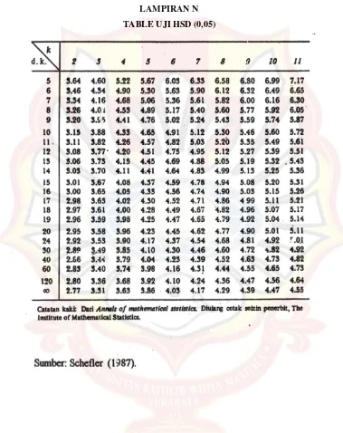
HASIL UJI STATISTIK KEKERASAN TABLET IBUPROFEN ANTAR FORMULA Interval for Mean

Min. Max.

Hipotesa pengujian :

(29)

KEKERASAN HSD

(I) F (J) F Mean Difference (I-J)

Std.

Error Sig.

95% Confidence Interval Lower Bound Upper Bound

I

II 1,03333 0,79546 0,230 -0,8010 2,8677

III 1,34000 0,79546 0,131 -0,4943 3,1743

IV 3,69333* 0,79546 0,002 1,8590 5,5277

II

I -1,03333 0,79546 0,230 -2,8677 0,8010

III 0,30667 0,79546 0,710 -1,5277 2,1410

IV 2,66000* 0,79546 0,010 0,8257 4,4943

III

I -1,34000 0,79546 0,131 -3,1743 0,4943

II -0,30667 0,79546 0,710 -2,1410 1,5277

IV 2,35333* 0,79546 0,018 0,5190 4,1877

IV

I -3,69333* 0,79546 0,002 -5,5277 -1,8590 II -2,66000* 0,79546 0,010 -4,4943 -0,8257 III -2,35333* 0,79546 0,018 -4,1877 -0,5190 Keterangan :

Symbol * : Perbedaannya signifikan, karena selisih > HSD (5%)

(30)

LAMPIRAN Q

HASIL UJI STATISTIK KERAPUHAN TABLET IBUPROFEN ANTAR FORMULA Interval for Mean

Min. Max.

(31)

KERAPUHAN

95% Confidence Interval Lower

(32)

LAMPIRAN R

HASIL UJI STATISTIK WAKTU HANCUR TABLET IBUPROFEN ANTAR FORMULA Interval for Mean

Min. Max.

(33)

WAKTU HANCUR

95% Confidence Interval Lower

(34)

LAMPIRAN S

HASIL UJI STATISTIK PERSEN OBAT TERLARUT TABLET IBUPROFEN ANTAR FORMULA

F Interval for Mean

Min. Max.

PERSEN OBAT TERLARUT PADA T = 30 MENIT

Source Sum of

Squares df Mean Square F Sig.

Between Groups 55,841 3 18,614 29,100 0,000

Within Groups 5,117 8 0,640

Total 60,959 11

(35)

PERSEN OBAT TERLARUT PADA T = 30 MENIT HSD

Keterangan :

Tanpa symbol : Perbedaannya tidak signifikan, karena selisih < HSD (5%) (I) F (J) F Mean

Difference (I-J) Std.

Error Sig.

(36)

LAMPIRAN T

HASIL ANAVA UJI KEKERASAN PADA PROGRAM DESIGN EXPERT

Response1Kekerasan

ANOVA for selected factorial model

Analysis of variance table [Partial sum of squares - Type III]

Sum of Mean F p-value

Source Squares df Square Value Prob > F

Model 22,35 3 7,45 7,99 0,0086 sig.

The Model F-value of 7,99 implies the model is significant. There is only a 0,86% chance that a "Model F-Value" this large could occur due to noise. Values of "Prob > F" less than 0,0500 indicate model terms are significant. In this case A, B are significant model terms.Values greater than 0,1000 indicate the model terms are not significant. If there are many insignificant model terms (not counting those required to support hierarchy), model reduction may improve your model.

Std. Dev. 0,97 R-Squared 0,7498

Mean 12,15 Adj R-Squared 0,6560

C.V. % 7,95 Pred R-Squared 0,4370

PRESS 16,78 Adeq Precision 6,686

The "Pred R-Squared" of 0,4370 is not as close to the "Adj R-Squared" of 0,6560 as one might

normally expect. This may indicate a large block effect or a possible problem with your model

and/or data. Things to consider are model reduction, response tranformation, outliers, etc.

(37)

Coefficient Standard 95% CI 95% CI

Final Equation in Terms of Coded Factors:

Kekerasan = +12,15

-1,01 * A

-0,86 * B

-0,34 * A * B

Final Equation in Terms of Actual Factors: Kekerasan = +12,14500

-1,00833 * Macam pengikat

-0,85500 * Macam penghancur

-0,33833 * Macam pengikat * Macam penghancur The Diagnostics Case Statistics Report has been moved to the Diagnostics Node.

In the Diagnostics Node, Select Case Statistics from the View Menu. Proceed to Diagnostic Plots (the next icon in progression). Be sure to look at the:

1) Normal probability plot of the studentized residuals to check for normality of residuals.

2) Studentized residuals versus predicted values to check for constant error. 3) Externally Studentized Residuals to look for outliers, i.e., influential values.

4) Box-Cox plot for power transformations.

(38)

LAMPIRAN U

HASIL ANAVA UJI KERAPUHAN PADA PROGRAM DESIGN EXPERT

Response2Kerapuhan

Sum of Mean F p-Value

The Model F-value of 32,20 implies the model is significant. There is only a 0.01% chance that a "Model F-Value" this large could occur due to noise. Values of "Prob > F" less than 0,0500 indicate model terms are significant. In this case A are significant model terms.Values greater than 0,1000 indicate the model terms are not significant. If there are many insignificant model terms (not counting those required to support hierarchy), model reduction may improve your model.

The "Pred R-Squared" of 0,8279 is in reasonable agreement with the "Adj R-Squared" of 0,8948.

"Adeq Precision" measures the signal to noise ratio. A ratio greater than 4 is desirable. Your ratio of 10,479 indicates an adequate signal. This model can be used to navigate the design space.

(39)

Coefficient Standard 95% CI 95% CI

Kerapuhan = +0,95

+0,57 * A

+0,039 * B

+2,500E-003 * A * B

Final Equation in Terms of Actual Factors: Kerapuhan = +0,94750

+0,57083 * Macam pengikat

+0,039167 * Macam penghancur

+2,50000E-003 * Macam pengikat * Macam penghancur The Diagnostics Case Statistics Report has been moved to the Diagnostics Node.

(40)

LAMPIRAN V

HASIL ANAVA UJI WAKTU HANCUR PADA PROGRAM DESIGN EXPERT

Response3Waktu Hancur

Model 341,58 3 113,861 22,04 < 0,0003 Sig.

The Model F-value of 22,04 implies the model is significant. There is only a 0,03% chance that a "Model F-Value" this large could occur due to noise. Values of "Prob > F" less than 0,0500 indicate model terms are significant. In this case A are significant model terms.Values greater than 0,1000 indicate the model terms are not significant. If there are many insignificant model terms (not counting those required to support hierarchy), model reduction may improve your model.

(41)

Coefficient Standard95% CI 95% CI

Waktu hancur = +15,58

+5,25 * A

-0,25 * B

-0,92 * A * B

Final Equation in Terms of Actual Factors: Waktu hancur = +15,58333

+5,25000 * Macam pengikat

-0,25000 * Macam penghancur

-0,91667 * Macam pengikat * Macam penghancur The Diagnostics Case Statistics Report has been moved to the Diagnostics Node.

(42)

LAMPIRAN W

HASIL ANAVA UJI PERSEN OBAT TERLARUT PADA T = 30 MENIT PADA PROGRAM DESIGN EXPERT

Response4Persen Obat Terlarut ANOVA for selected factorial model

Model 55,58 3 18,61 29,10 < 0,0001 Sig.

The Model F-value of 29,10 implies the model is significant. There is only a 0.01% chance that a "Model F-Value" this large could occur due to noise. Values of "Prob > F" less than 0,0500 indicate model terms are significant. In this case A, B, AB are significant model terms.Values greater than 0,1000 indicate the model terms are not significant. If there are many insignificant model terms (not counting those required to support hierarchy), model reduction may improve your model.

(43)

Coefficient Standard 95% CI 95% CI

Final Equation in Terms of Coded Factors: Persen obat terlarut = +94.97

-1.74 * A

+0.82 * B

-0.97 * A * B

Final Equation in Terms of Actual Factors: Persen obat terlarut = +94.97417

-1.74417 * Macam pengikat

+0.81583 * Macam penghancur

-0.97250 * Macam pengikat * Macam penghancur The Diagnostics Case Statistics Report has been moved to the Diagnostics Node.

(44)

LAMPIRAN X

HASIL UJI STATISTIK HASIL PERCOBAAN DAN HASIL TEORITIS PADA UJI KEKERASAN

Paired Samples Statistics

Paired Samples Correlations

N Correlation Sig.

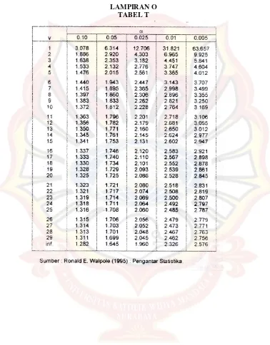
Percobaan & Teoritis 4 1,000 0,000

Paired Samples Test Paired Differences

t df Sig. (2-tailed)

Mean Std.

Deviation Std. Error Mean

95% Confidence Interval of the

Difference Lower Upper Percobaan

- Teoritis 0,0050 0,0238 0,0119 -0.0329 0,0429 0,42 3 0,703

Mean N Std. Deviation Std. Error

Mean

Percobaan 12,1550 4 1,5590 0,7795

(45)

LAMPIRAN Y

HASIL UJI STATISTIK HASIL PERCOBAAN DAN HASIL TEORITIS PADA UJI KERAPUHAN

Mean

Percobaan 0,9500 4 0,6652 0,3326

Teoritis 0,9500 4 0,6598 0,3299

Mean Std.

(46)

LAMPIRAN Z

HASIL UJI STATISTIK HASIL PERCOBAAN DAN HASIL TEORITIS PADA UJI WAKTU HANCUR

Mean

Percobaan 15,5850 4 6,1603 3,0802

Teoritis 15,5800 4 6,1613 3,0807

Mean Std.

(47)

LAMPIRAN AA

HASIL UJI STATISTIK HASIL PERCOBAAN DAN HASIL TEORITIS PADA UJI PERSEN OBAT TERLARUT PADA T = 30

MENIT

Mean

Percobaan 94,9775 4 2,4901 1,2450

Teoritis 94,9700 4 2,4875 1,2438

Mean Std.

(48)

LAMPIRAN AB

UJI F KURVA BAKU PENETAPAN KADAR

Uji Kesamaan Regresi (NaOH) Konsentrasi

Σ 906363,64 2,563276 1523,946

Konsentrasi

400,4 0,682 160320,16 0,465124 273,0728

500,5 0,838 250500,25 0,702244 419,419

600,6 0,993 360720,36 0,986049 596,3958

Σ 911820,91 2,565498 1529,2277

Konsentrasi

399,6 0,678 159680,16 0,459684 270,9288

499,5 0,837 249500,25 0,700569 418,0815

599,4 0,996 359280,36 0,992016 597,0024

(49)

Σ X2 _{Σ XY} _{Σ Y}2

N SSi RDF

Regresi I Regresi II Regresi III

906363,6400 1523,9460 2,563276 6 0,00093644 4 911820,9100 1529,2277 2,565498 6 0,00080867 4 908180,9100 1522,1763 2,551605 6 0,00032841 4

Σ 2726365,46 4575,35 7,680379 0,002087909

Ssc = 0,002073527

(50)

LAMPIRAN AC

UJI F KURVA BAKU UJI DISOLUSI

Uji Kesamaan Regresi (Dapar Fosfat pH 7,2) Konsentrasi

500,5 0,909 250500,25 0,826281 454,9545

600,6 1,014 360720,36 1,028196 609,0084

Σ 911820,91 2,812563 1600,599

Konsentrasi

400,4 0,722 160320,16 0,521284 289,0888

500,5 0,919 250500,25 0,844561 459,9595

600,6 1,092 360720,36 1,192464 655,8552

Σ 911820,91 3,020955 1659,658

Konsentrasi

400,8 0,721 160640,64 0,519841 288,9768

501 0,912 251001 0,831744 456,912

601,2 1,09 361441,44 1,1881 655,308

(51)

Σ X2 _{Σ XY} _{Σ Y}2

N SSi RDF

Regresi I Regresi II Regresi III

911820,91 1600,599 2,812563 6 0,002891571 4 911820,91 1659,658 3,020955 6 0,00011544 4 913643,64 1657,7088 3,00785 6 0,00011444 4

Σ 2737285,46 4917,9658 8,841368 0,005465438

Ssc = 0,005465438

F hitung = 3,003715147 < Ftabel 0,05(3;12) 3,49