www.elsevier.nl / locate / econbase
When is two better than one? How federalism mitigates
and intensifies imperfect political competition
Bryan Caplan
Department of Economics and Center for Study of Public Choice, George Mason University, Fairfax, VA 22030, USA
Received 1 February 1999; received in revised form 1 February 2000; accepted 1 February 2000
Abstract
The current paper models power-maximizing politicians’ behavior subject to imperfect political competition and perfect citizen mobility. It then analyzes the welfare implications of federal and non-federal structures. The model abstracts from both heterogeneous preferences (the most common argument in favor of federalism) and externalities (the most common argument against), showing that even in this simplified setting federalism has important welfare implications. There is one class of equilibria in which more federalism has the purely beneficial effect of offsetting imperfections in the political process. However, there is also a second class of equilibria in which citizen mobility makes political imperfections more severe by creating ‘safe districts’ for both political parties. 2001 Elsevier Science B.V. All rights reserved.
Keywords: Optimal federalism; Imperfect political competition; Intergovernmental competition
JEL classification: D72; H11; D60
1. Introduction
State and local politicians find themselves constrained by both politics — most notably, the need to win elections — and economics — most notably, the option of dissatisfied customers to go elsewhere with their human and / or physical capital. The welfare analysis of subjecting politicians to democratic voting — especially
E-mail address: [email protected] (B. Caplan).
relative to dictatorship — has been largely favorable (Wittman, 1989, 1995; McGuire and Olson, 1996). But the welfare analysis of the relocation option has been more equivocal. As Rose-Ackerman (1983) puts it, ‘‘A multiple-government system has little normative appeal if everyone has the same tastes and incomes and if the government apparatus is controlled by voters.’’ (pp. 25–26). Even when there is substantial heterogeneity of tastes, this must be weighed against the inability of decentralized governments to cope with interjurisdictional externalities (Gordon, 1983; Donahue, 1997). Inman and Rubinfeld (1996) contrast this ‘optimal tax’ account of federalism to the ‘political economy’ view. While the former treats governments as faithful agents of their citizens, the political economy perspective emphasizes that federalism helps mitigate the principal-agent problems of democracy (Brennan and Buchanan, 1980; Frey and Eichenberger, 1996; Inman and Rubinfeld, 1997; Qian and Weingast, 1997).
The current paper formally shows that even abstracting from heterogeneous
preferences and interjurisdictional externalities, federalism can both improve and
worsen the performance of democratic governments. I develop a model in which politicians compete electorally with another party within their state, and compete economically with a rival government outside their state. As in Lindbeck and Weibull (1987), Grossman and Helpman (1996), and Dixit and Londregan (1995, 1996, 1998a,b), elections work imperfectly: voters treat parties as differentiated products. This model is rich enough to generate two quite different classes of equilibria. In the first class, the need to keep citizens from moving away leads politicians to improve their policies even if they are electorally secure. Federalism then mitigates the impact of the dominant party’s monopoly power. In the second class of equilibria, however, the loyalists of each party tend to move to the state their party is expected to control. This process makes the political imperfections in both states more severe.
The next section describes the players and their objective functions. The third section solves the model and welfare ranks the possible equilibria. The fourth section examines the robustness of these findings to alternate assumptions. The fifth section analyzes the practical significance of the results. The sixth section concludes.
2. Players, preferences, and the benchmark equilibrium
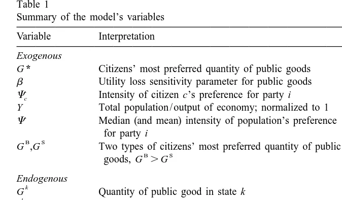
Table 1
Summary of the model’s variables Variable Interpretation Exogenous
*
G Citizens’ most preferred quantity of public goods
b Utility loss sensitivity parameter for public goods
Cc Intensity of citizen c’s preference for party i Y Total population / output of economy; normalized to 1
C Median (and mean) intensity of population’s preference for party i
B S
G ,G Two types of citizens’ most preferred quantity of public
B S
goods, G .G Endogenous
k
G Quantity of public good in state k k
zc Indirect utility function of citizen c in state k k
I Indicator variable51 if party i wins in state k, 0 otherwise k k
u ,ui j Utility function of state parties i, j in state k k
Y Total population / output in state k k
*
d Squared deviation of G in state k k
C The median of the distribution ofCcin state k
1. All citizens must vote for their most-preferred party in their state.
2. All political parties must offer platforms that maximize their expected utility. 3. All citizens must reside in their most-preferred state (if they have a choice). If
they are indifferent between states they randomize with equal probabilities.
2.1. Citizens
Total wealth is assumed to be the same for all citizens, and is also normalized to equal 1. Citizen utility depends upon not only consumption of private and public goods, but also on the political environment. These tastes and the per-capita budget constraint yield citizens’ indirect utility function, assumed to be of the following form:
k k 2 k
*
zc5 2b(G 2G ) 1CcI . (1)
*
G is citizens’ most-preferred per-capita size of government; the assumption of homogeneous policy preferences makes the positive and negative role of
federal-k
[20.51C, 0.51C], whereC .0 is both the average and the median value of
Cc.
There are a couple ways to interpretCc. Lindbeck and Weibull (1987) suggest that it captures parties’ contrasting and relatively fixed commitments to important non-economic policies, such as their stances on abortion and national defense. While most of the current paper assumes that both share the same power-maximizing objective, this does not rule out the possibility of different objectives
1
along other margins. Alternately, in line with much of the empirical political science literature on party affiliation (e.g., Mutz and Mondak, 1997; Sears et al., 1980; Luttbeg and Martinez, 1990), Cc could irreducibly reflect individuals’ inherited partisan loyalties. Just as many sports fans root for ‘their’ team even though all teams have the same objective function, many voters strictly prefer ‘their’ party even if it acts the same as its competitor. For example, Catholic voters might continue voting for traditionally preferred Democratic candidates even though platform changes leave them somewhat ideologically closer to Repub-licans. While such advantage erodes over time, the erosion may be so gradual that for practical purposes each generation of politicians treats its level as fixed.
2.2. Parties
Controversy still surrounds political parties’ objective functions. In Grossman and Helpman (1996) and Dixit and Londregan (1995, 1996, 1998b), political
2
parties’ objective is to maximize their votes. Dixit and Londregan’s (1998a) parties maximize a weighted average of votes and an ideological social welfare function; Alesina and Rosenthal (1995) similarly assume that parties advance divergent ‘leftist’ and ‘rightist’ ideologies subject to electoral constraints. In contrast, both Brennan and Buchanan (1980) and McGuire and Olson (1996)
3
assume they seek to maximize their own power. Caplan (1999a) presents empirical evidence on the relative merits of the ideological and power-maximizing views of party motivation, finding that both theories have some validity. The core of this paper builds on the power-maximizing assumption because it makes the
1
More importantly, a later section shows that the simple model’s results still hold when competing parties have different policy objective functions.
2
On the theory of politicians with preferences over both policies and electoral victory, see Wittman (1983).
3
model more tractable and the results clearer: unlike ideological parties, all power-maximizing parties want to shirk in the same way. Yet power-maximization is not necessary for the main results: Section 4 shows that if parties have divergent ideologies, the modified model is nearly isomorphic. The power-maximizing motive of the parties is formalized by assuming that parties’ utility increases monotonically as the size of government they control grows:
k k k k
ui5I G Y ,i (2)
k k k k
uj5(12I )G Y ,j (3)
k k
where G and G are the political platforms offered in state k by parties i and j.i j
2.3. The benchmark regime: politicians constrained solely by elections
Suppose a regime has democratic elections, but citizens and their wealth cannot move to another locality. Each state has demographically identical populations of 0.5 irrespective of policy. This lack of mobility could be interpreted as a system of immigration controls, or as the result of a federal tax and grant system that leaves
k k
no incentive for relocation at the margin. Using (1), and defining d ;(G 2
2
*
G ) , it can be seen that citizens vote for party i if
k k
2bd 1C $ 2 bdi c j, (4)
and for party j otherwise. Similarly, the political parties only need to worry about beating each other, so (2) and (3) become
k k k
ui50.5I G ,i (5)
k k k
uj50.5(12I )G .j (6)
Given majority rule, it will then not be an equilibrium for both political parties to offer the median preference. Since by assumption C .0, party i wins with
*
certainty if it plays G . Party i will want to keep increasing the offered level of government until it drives the percentage of votes it receives down to 0.5, leaving the median voter indifferent:
k k
C 2 b(d 2 di j)50. (7)
Due to disadvantaged status, in equilibrium party j will never win. However, neither party will have an incentive to change its behavior only if j minimizes i’s votes by making the median voter as well-off as possible:
k k
minC 2 b(d 2 di j). (8)
k
k
*
Solving (8) reveals that j’s vote-maximizing strategy is to set Gj5G . One can
k
*
find i’s best response by plugging Gj5G into (7), yielding
]
In the benchmark equilibrium, then, the party with the greater political advantage always wins, but is constrained in its choices by the presence of the alternative, less popular party. The disadvantaged party offers to set the size of government equal to citizens’ bliss point. The advantaged party’s deviation from citizens’ most-preferred level is an increasing function of the magnitude of the political advantage of the dominant party divided by the loss-sensitivity parameter. It goes as far as it can get away with without losing office.
2.4. Welfare analysis of the benchmark regime
Treating Cc as a random variable, one can calculate total citizens’ expected utility in a given regime. In general,
1 1 2 2
E(z )c 5Y E(z )c 1Y E(z ).c (10)
k
Using (1), definingC as the median value ofCc in state k, and noting that the median and mean value ofCc are equal:
1 1 1 1 2 2 2 2
E(z )c 5Y (2bd 1C I )1Y (2bd 1C I ). (11)
Computing citizens’ expected utility in the benchmark regime is straightforward.]]
k k k k
*
Gi5G 1
œ
C/b, Y 50.5 andC 5C since there is no mobility, and I 51 since party i controls both states. Substituting these into (11) reveals that thebenchmark utility level is 0 :
] 2
C ]
E(z )c 5 2b
S D
œ
b 1C 50. (12)3. Political equilibrium and welfare with both mobility and voting
This section characterizes the equilibria of the game with both free elections and unconstrained mobility, then compares the expected utility of these equilibria to
k k k
that of the benchmark regime. Y ,C , and I become endogenous functions of policy, as one would expect for members of democratic federal systems. Unlike the simplified game without mobility, which has the unique benchmark equilib-rium, the more complex game with both voting and mobility can have multiple
k
equilibria. These are possible because unrestricted movement directly affectsC , the median of the distribution ofCc in state k, which in turn influences political
1 2
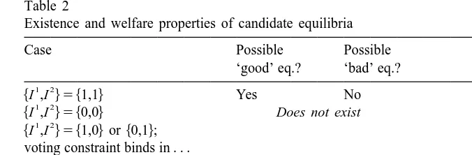
Table 2
Existence and welfare properties of candidate equilibria
Case Possible Possible voting constraint binds in . . .
. . . neither state Yes Yes
. . . state 2 but not state 1 Yes Yes . . . both states Does not exist . . . state 1 but not state 2 Does not exist
h1,0j, or h0,1j. Table 2 summarizes this section’s results, dividing equilibria into ‘good’ equilibria where expected utility is weakly greater than the benchmark level, and ‘bad’ equilibria where it is strictly lower.
1 2
3.1. Party i wins in both states: hI ,I j5h1,1j
If party i is expected to win in both states, there is no incentive to relocate on
k
the basis of partisan preferences, soC 5C. Whichever state has the lower value
k
ofd accordingly gets 100% of the population. As in the Bertrand duopoly game, this leaves only one Nash equilibrium in which the ruling party in both states sets
k
d 50. Both states get exactly half the population. To sustain this equilibrium, both chapters of party i need merely ensure that they win elections in both states.
k
As shown in Section 2.3, party i can always win the election ifC .0, so an
1 2
equilibrium with hI ,I j5h1,1j always exists.
Expected utility in this regime is clearly higher than in the benchmark case, which has expected utility of 0. Using (11):
1 1 1 1 2 2 2 2
E(z )c 5Y (2bd 1Ci I )1Y (2bd 1Ci I )
50.5(01C)10.5(01C)5C .0. (13) Hence, this is always one of the ‘good’ equilibria where mobility makes democracy work better. Note further that there is no reason to regard this as an unstable equilibrium, as identical communities can be in a simple Tiebout model with heterogeneous citizens. In a world with small random perturbations, the i parties would adjust by aiming for a larger victory margin.
1 2
3.2. Party j wins in both states: hI ,I j5h0,0j
If party j is expected to win in both states, there is no incentive to relocate on
k
the basis of partisan preferences, so C 5C. As shown in Section 2.3, this
k
1 2
3.3. Party i wins in one state, party j wins in the other: hI ,I j5h1,0j or h0,1j
The numbering of the states is arbitrary, so the equilibrium conditions for
1 2 1 2
hI ,I j5h1,0jandhI ,I j5h0,1jare essentially identical. For simplicity, then, this
1 2
section looks only athI ,I j5h1,0j, where party i wins in state 1 and party j wins in state 2.
In any equilibrium, note that citizens in state k are indifferent between voting for i and j when
k k
C 5 bc (d 2 di j). (14)
Note further that in any equilibrium, the median voter must weakly prefer the
*
winner, and losing parties’ platforms set the size of government equal to G . Using (14) and these two facts permits the derivation of both electoral victory constraints:
1 1
bd #Ci , (15)
2 2
bd # 2Cj . (16)
Citizens are indifferent between living under i in state 1 and under j in state 2 when
dj) strictly prefer state 2. The fraction of citizens in each state is thus given by
1 1 2
Y 50.51C 2 b(d 2 di j), (18)
2 1 2
Y 50.52C 1 b(d 2 di j). (19)
The demand for residence in state 1 is (a) an increasing linear function of the mean preference for party i over party j, (b) a decreasing function of the deviations from voters’ bliss points in state 1, and (c) an increasing function of the deviations from voters’ bliss points in state 2. The opposites hold for residence in state 2.
The median value ofCc in both states can be derived from the distributions implied by (18) and (19):
1 2
Plugging (20) into (15) and (21) into (16) yields i’s electoral victory constraint in state 1 and j’s corresponding constraint in state 2:
1 2
bd #i 0.51C 2 bdj, (22)
2 1
bd #j 0.52C 2 bdi. (23)
To understand the welfare properties of this class of equilibria, plug (18)–(21) into (11) to get an expression for citizens’ expected utility:
1 2
0.51C 1 b(d 2 di j)
1 2
F
1H
JG
]]]]]]]
E(z )c 5h0.51C 2 b(d 2 di j)j 2bd 1 2
1 2 2
1h0.52C 1 b(d 2 di j)j[2bd ], (24)
which reduces to
1 2 2 1 2 1 2
E(z )c 50.5[b(d 2 di j)] 2C[b(d 2 di j)]20.5[b(d 1 di j)]
2
10.5[C 1C 10.25]. (25)
In principle, there are four sub-cases to consider: (a) the voting constraint binds in neither state; (b) the voting constraint binds in state 2 but not state 1; (c) the voting constraint binds in both states; (d) the voting constraint binds in state 1 but not state 2. Simple proofs by contradiction show that sub-cases (c) and (d) never exist. In contrast, it can be proven that both equilibria (a) and (b) are possible, and may be either welfare-superior or inferior to the benchmark. All of these proofs appear in Appendix A. The remainder of this section provides an intuitive discussion of equilibria (a) and (b) and their welfare properties, and offers some illustrative examples.
1 2
The novel feature of the equilibria where hI ,I j5h1,0j is that both parties simultaneously rid themselves of the most hostile elements of their electorates. This allows either one or both parties to set per-capita government spending at the
k k
value that maximizes G Y without fear of electoral consequences. It remains true that ruling parties attract more population and increase their vote share when their policies improve. But with the least-friendly voters safely in the rival state, political competition becomes weaker in both jurisdictions.
Two opposing forces thus make the welfare properties of these equilibria ambiguous. On the positive side, when i rules in one state and j rules in the other, no one has to suffer under the rule of the party they dislike. This is especially beneficial for extreme partisans. On the negative side, when i rules in one state and
j rules in the other, equilibrium policies tend to worsen because political
3.3.1. Voting constraint binds in neither state
It is easiest to understand the equilibrium where the voting constraint binds in neither state by relaxing the assumption that C .0 and setting C 50. Then elections function perfectly competitively so long as the entire electorate — or a representative sample thereof — participates. But with mobility, the electorate in each state is a self-selected and therefore unrepresentative sample. Voters with positiveCc tend to live in state 1, and voters with negativeCc tend to live in state 2, so political competition becomes imperfect — and policy gets worse — in both states. But from the point of view of citizen welfare, the crucial question is: how much worse? ‘Matching’ citizens with their preferred parties is clearly an advantage from a welfare standpoint. If policy only gets a little worse, then the net effect on welfare will still be positive. If policy gets much worse, however, welfare falls.
What then determines how much policy quality deteriorates? As Eq. (A.6) in Appendix A shows, when C 50, the unconstrained equilibrium deviation is a simple function of two variables: the sensitivity parameter b and the bliss point
* *
G . As either variable grows, parties’ departures from G decrease, so
equilib-] Œ]
*
rium deviations from voters’ ideal point fall. At the critical point G
œ
b 51 / 8, the welfare costs of imperfect political competition and the welfare gains of matching exactly balance each other, leaving expected utility at the benchmark]
*
level. For higher values of G
œ
b, welfare exceeds the benchmark level; for lower values, it falls short of it.Table 3 illustrates the fact that this can be either a ‘good’ or a ‘bad’ equilibrium.
*
For the low values of G and b, the equilibrium is welfare-inferior to the
*
benchmark. For the intermediate value shown in the table, the product of G and
]
Œ
b is precisely 1 / 8; welfare is consequently exactly equal to the benchmark level. For considerably larger values of the two crucial parameters, welfare exceeds the benchmark level. With mobility high, and the desired level of government large to begin with, the quality of policy causes little harm compared to the benefits of matching.
3.3.2. Voting constraint binds in state 2 but not state 1
Now take the case where the voting constraint does bind in state 2, but not state
1
1. As Appendix A shows, for small values ofbdi or large values ofC, expected utility exceeds the benchmark level. When C takes on smaller values, welfare
Table 3
Parameter values and welfare for equilibrium 3.3.1
1 2
*
b G bdi bdj E(z )c
1 0.1 0.205 0.205 20.16
2 0.25 0.125 0.125 0
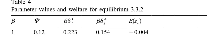
Table 4
Parameter values and welfare for equilibrium 3.3.2
1 2
b C bdi bdj E(z )c
1 0.12 0.223 0.154 20.004
6 0.12 0.192 0.188 0.002
1 0.2 0.226 0.074 0.076
6 0.2 0.196 0.104 0.081
1 1
properties depend on the size ofbdi. For small values ofbdi, welfare exceeds the benchmark level; for large values, the benchmark is welfare superior.
How can this be interpreted intuitively? Using (22) and (23), consider two salient features of equilibria where the voting constraint binds in state 2 but not state 1. First, the deviation in state2 will be smaller than the deviation in state 1. If the deviation is small in state 1, the deviation in state 2 must be smaller still.
1
Thus, when bdi is small, policies must be good in both states, no one is trapped under the rule of a party they strongly dislike, and welfare in higher than in the benchmark case. Second, asC increases, summed policy deviations must decline. WhenC is large, good policies in state 2 tend to counter-balance bad policies in state 1. For C .0.125, this effect is strong enough to guarantee that welfare
1
exceeds the benchmark level. In contrast, whenC is small andbdi is large, policy will be bad in both states, and welfare falls below the benchmark level: the social costs of bad policy then outweigh the social benefits of better satisfaction of conflicting party loyalties.
*
To illustrate these points, suppose we fix G 50.1, and note how the equilibrium and its welfare properties change asb andC vary (Table 4). For the
1
smaller value,C 50.12, the welfare properties hinge on the value ofbdi, which
*
in turn depends onb, the sensitivity of utility to deviations from G . Whenb rises
1
from 1 to 6, the equilibrium value of bdi falls, and expected utility rises from somewhat below the benchmark level to somewhat above. In contrast, for the larger value,C 50.2, welfare always exceeds the benchmark level.
4. Robustness of the model
change. The following six sections examine how changing one assumption at a time in the basic model — keeping all of the others fixed — alters the results.
4.1. Opposing ideologies
In my model, both parties maximize the size of government. A more common modeling strategy, however, is to assume that parties have opposing ideologies, such as ‘small government’ versus ‘big government.’ Suppose, then, that party j’s objective function is still given by (3), but party i’s utility is an increasing function of the size of the private sector conditional on holding power:
k k k k
ui5I (12G )Y .i (29)
Since the critical variable is squared equilibrium deviations from voters’ ideal point, a surprising fraction of the model’s results go through nearly unchanged. In the simplified version of the model without mobility, i deviates as far as possible
k
from voter preferences as it can without losing office, so di remains C/b. The only difference is in the direction of deviation: (9) becomes:
] C k
]
*
Gi5G 2
œ
b. (99)For the equilibrium with both voting and mobility, it is apparent that Eqs.
*
(15)–(23), being symmetric with respect to deviations from G , do not change. It
*
is only necessary to remember that party i deviates below G , while j deviates above. Thus, the results for Sections 3.1 and 3.2 go through unchanged. The key conclusions for Section 3.3 are likewise robust, though the details of the analysis
5
must be slightly modified.
4.2. Heterogeneous policy preferences
Most models of federalism assume that citizens have diverse tastes about policy,
*
not a single shared G as the current paper does. Suppose then that there are equal proportions of two types of voters, one whose most-preferred size of government
B S B S
is G while the other’s is G , with G .G . The voters are otherwise identical; in
particular, for both types, the distribution ofCcis the same. The set of equilibria of this modified version of the model is complex because both the distribution of policy preferences as well as the distribution ofCc are endogenous. An appendix, available from the author, discusses the most straightforward cases, and shows that with heterogeneous preferences there are still ‘good’ and ‘bad’ equilibria.
5
4.3. Moving costs and initial citizen distribution
In the version of the model in Section 2, moving costs are effectively infinite. In Section 3, mobility is costless. What about intermediate cases? An earlier version of this paper shows that most of the results from Section 3 persist. The main difference is that, with mobility costs, inter-jurisdictional competition is imperfect. Even when party i rules in both states, mobility cannot pressure parties to offer
*
G . The welfare analysis is largely unchanged; the main difference is that it is
necessary to take account of realized mobility costs when calculating the net welfare impact of federalism (Caplan, 1999b).
With positive mobility costs, the initial distribution of citizens begins to matter too. In general, a less-than-perfectly-evenly-distributed population enhances the advantages of federalism. The disadvantage of federalism is that citizens with similar party preferences cluster together, leading to weak political competition. If citizens with similar party preferences are initially clustered, however, the marginal disadvantages of mobility decline and the marginal advantages increase. In effect, if citizens cluster ex ante, the relevant ‘benchmark’ equilibrium’s welfare level is lower, so it is more likely that the equilibrium with mobility is welfare-superior.
4.4. More jurisdictions
Increasing the number of jurisdictions, while retaining the assumption of costless mobility, can yield a first-best outcome. With four jurisdictions, there exists an equilibrium where party i rules in two states, party j rules in the other
*
two, the equilibrium level of government in all four states is G , and everyone lives under their most-preferred political party. In general, so long as there is costless mobility, if one party rules any two states, mobility pressures both to set
*
the size of government to G . Mobility costs naturally tend to weaken this result, as do heterogeneous policy preferences.
4.5. Coordination
4.6. Timing and commitment
The model assumes that all players make their moves simultaneously. In this case, there can be no commitment problem. Altering this timing assumption could clearly modify the game’s results, particularly if parties possess no credible commitment technology. If people make their location decisions first, and parties subsequently set policy, then at the time of decision, elections are the only factor constraining parties’ platforms.
The model must then be solved by backwards induction. Note that, in equilibrium, voting constraints must bind in both states, so there are only two cases that need to be analyzed. In the first, i wins in both states, and sets
]]
1 2
Gi5Gi5
œ
C/b. The welfare level is no different from that without mobility. In the second, i wins in one state, and j wins in the other. In this case, (15) and (16)1 1 2 2
reduce to: bd 5Ci and bd 5 2Cj . Substituting these values into (20) and
1 2
(21) and solving forC andC reveals that this equilibrium exists only ifC 50. While the model’s findings are definitely sensitive to the timing assumption, moving to a repeated game structure would probably restore the relevance of the results for the simultaneous game. Given sufficiently low discount rates, the ‘cooperative’ solution — where parties implement promises they make prior to citizens’ location decisions — should be sustainable. Parties would not take advantage of one turn’s electoral slack because this would reduce their state’s population in subsequent turns.
5. Implications for federalism
The importance of heterogeneous preferences as an argument for decentraliza-tion, and interstate spillovers as an argument against, appears repeatedly in the optimal federalism literature. As Gordon (1983) argues:
There may be advantages to decentralizing government decision-making. Local governments, being ‘closer to the people,’ may better reflect individual preferences. The diversity of policies of local governments allows in-dividuals to move to that community best reflecting their tastes. Competition among communities should lead to greater efficiency and innovation. However, this paper has shown the many ways in which decentralized decision-making can lead to inefficiencies, since a local government will ignore the effects of its decisions on the utility levels of nonresidents (p. 584).
notable result is that there are ‘good’ equilibria where mobility mitigates political imperfections and ‘bad’ equilibria where mobility intensifies them (Table 2). Even in a world where citizens’ policy tastes were uniform and state policies affected only residents, federalism is not necessarily useless — or necessarily beneficial.
5.1. The ‘good’ equilibria
The intuition behind the ‘good’ equilibria is straightforward: if politicians take excessive advantage of imperfect political competition, citizens leave. Power-maximizing politicians may therefore moderate their excesses not because they fear electoral defeat, but because population outflows reduce their power. If politicians win supermajorities by doing exactly what citizens want, they have an incentive to make government bigger; if the supermajority is ample enough, the ruling party will even have a supermajority at the unconstrained maximum value
k k k
of G Y . At that point there is no longer any reason to make G larger because iti i k k
cuts both the winning party’s share of the vote and G Y .i
State and local governments in federal democracies usually face both political and economic constraints. This might indicate that constitutional framers think that the ‘good’ equilibria are empirically predominant; if the framers foresee imperfect electoral competition, they can mitigate it by sub-dividing the polity. In this case, Brennan and Buchanan (1980) are correct to argue that that inter-jurisdictional competition reduces the power of Leviathan.
5.2. The ‘bad’ equilibria
But matters are more complicated: the interaction of mobility and imperfect political competition can also make the monopoly power of government greater. The underlying intuition is that if voters with opposite party tastes divide up into their own ‘safe districts,’ then competitive elections may be absent in every state. If a politician implements bad policies, the first people to exit are those who most dislike the current office-holders. This shifts the absolute value of median party tasteCc further from zero, making worse policies electorally sustainable. This is possible because living under one’s preferred political party is a private good, but the welfare properties of the political equilibrium are a public good. Perfect sorting of citizens according to the sign ofCc maximizes the realized sum of citizens’
party preferences, but at the same time makes policy imperfections as large as
possible.
only do the political imperfections in San Francisco become more severe; at the same time, the staunch Republicans who move to Republican districts also exacerbate the political imperfections in their new localities. The ‘bad’ equilibria offer a novel explanation for why voters may simultaneously dislike incumbents’ policies, yet continue to vote for them: they have self-selected into districts with strong partisan loyalties. Rational power-maximizing politicians take advantage of the situation by deliberately deviating from voters’ policy preferences. So long as the reigning politicians’ deviation from voter preferences does not exceed the median degree of party loyalty, the political machine can stay in power indefinitely.
What is particularly interesting about the ‘bad’ equilibria is that they can emerge even if C 50, i.e. if the median voter in the overall population has no party preference whatever. If voters expect i to win in one state and j in the other, it makes sense for people withC .c 0 to move to the state where i rules, and for the people with C ,c 0 to move to the state where j rules. Imperfect political competition itself can therefore arise endogenously because a balanced population tends to sub-divide into two imbalanced populations. It is therefore unnecessary to assume that the distribution of Cc is skewed towards one party to generate imperfect political competition.
5.3. Interpreting the model
6. Conclusion
The model presented in this paper appears to be the first in which citizens’ mobility endogenizes political imperfections. It is intended not as a substitute to but as a complement for the more traditional approach to optimal federalism (Gordon, 1983), showing that there are additional arguments for and against federalism when political competition works imperfectly. There are ‘good’ equilibria where citizen mobility dampens the importance of imperfect political competition, and ‘bad’ equilibria where citizen mobility creates ‘safe districts,’ in which the political process is even less competitive.
There are several possible outlets for further research building on this paper’s insights. While the model is relatively simple, it shows that citizen migration and political imperfection can interact in sometimes unexpected ways. These may be of some practical importance in understanding, for example, the recent waves of secessions and political and economic unions. Since the model can give rise to both ‘good’ and ‘bad’ equilibria for the same set of parameters, further examina-tion of the condiexamina-tions under which federalism mitigates imperfect political competition is also in order. The widespread use of federalist institutions perhaps suggests that the ‘good’ equilibria occur most frequently. On the other hand, continuing dissatisfaction with the performance of government might be a sign that voters are stuck in a ‘bad’ equilibrium in which citizen mobility has amplified the inherent imperfections of the political process.
Acknowledgements
I would like to thank my advisor, Anne Case, as well as Igal Hendel, David Bradford, Robert Willig, Harvey Rosen, Alessandro Lizzeri, Gordon Dahl, Sam Peltzman, Tom Nechyba, Tyler Cowen, Bill Dickens, Yesim Yilmaz, Roger Gordon, David Levy, Robin Hanson, two anonymous referees, and seminar participants at Princeton and George Mason for numerous helpful comments and suggestions. Gisele Silva provided excellent research assistance. The standard disclaimer applies.
1 2
Appendix A. Party i wins in one state, party j wins in the other: hI ,I j5
h1,0j orh0,1j
Voting constraint binds in neither state
1 1
Party i in state 1 maximizes G Y subject to (18):i
1 1 2
max Gih0.51C 2 b(d 2 di j)j. (A.1)
1
Gi
Differentiating (A.1) and setting it equal to zero:
1 2 1 1
The analogous equation for j’s best response is
]]]]]]]]]2 1
Considering the special case where C 50 is sufficient to show that this equilibrium can be welfare-superior or welfare-inferior to the benchmark case, depending on parameter values. Then there is a simple symmetric equilibrium,
1 2 Recall that the expected utility of the benchmark is 0. Using (25), it can be seen that utility equals the benchmark level iff
1 2 2 1 2 1 2 2
[b(d 2 di j)] 22C[b(d 2 di j)]2[b(d 1 di j)]1[C 1C 10.25]50. (A.7)
If the left-hand side of the above expression is greater than zero, this equilibrium is better than the benchmark; if less than zero, worse. Plugging into (A.7), it can be seen that expected utility exceeds that of the benchmark iff
Voting constraint binds in state 2 but not state 1
In this case, (A.3) still holds for party i. Since (23) binds, it may be used to substitute out for party j’s strategy:
]]]]]]]]]]]]]]]2 1
Plugging (A.13) back into j’s constraint:
]]]]]2 2
To analyze welfare, recall that because (23) binds:
1 2
b(d 1 di j)50.52C. (A.15)
Substituting (A.15) into (A.3) and re-arranging terms implies
1 2 2 1 2 2
[b(d 2 di j)] 22C[b(d 2 di j)]1C 12C 20.2550. (A.16)
Note that for values ofC .0.125, the left-hand side of (A.16) is always positive. (A.16) has two real solutions:
]] Œ128C
1 2
]]]
[b(d 2 di j)]5C 6 2 . (A.17)
From (A.13) and (A.14), we know that
]]]]]2 2
Combining (A.17) and (A.18), and simplifying:
Note, however, that the left-hand-side of (A.19) is bounded between 0 and 0.25, and the benchmark offer the same expected welfare levels. It is welfare-superior to
]]
1 Π1
the benchmark iff bd ,i (12 128C) / 4, and welfare-inferior if bd .i (12 ]]
Œ128C) / 4.
Voting constraint binds in both states
Proof by contradiction shows this equilibrium will never exist. Suppose it did: Then (22) and (23) both hold with equality. This implies thatC 50, which is a contradiction since by assumptionC .0.
Voting constraint binds in state 1 but not state 2
Proof by contradiction shows this equilibrium will never exist. Suppose it did: then (22) holds with equality, while (23) holds as a strict inequality. Plugging the
2 2
equality into the inequality implies:bd ,j 0.52C 2[0.51C 2 bdj]. Cancelling terms leaves 0, 22C, which is a contradiction sinceC .0.
References
Alesina, A., Rosenthal, H., 1995. Partisan Politics, Divided Government, and the Economy. Cambridge University Press, New York.
Brennan, G., Buchanan, J.M., 1980. The Power to Tax: Analytical Foundations of a Fiscal Constitution. Cambridge University Press, Cambridge.
Caplan, B., 1999a. Has Leviathan been bound? A theory of imperfectly constrained government with evidence from the States. Unpublished manuscript, George Mason University.
Caplan, B., 1999b. When is two better than one? How federalism mitigates and intensifies imperfect political competition. Unpublished manuscript, George Mason University.
Dixit, A., Londregan, J., 1995. Redistributive politics and economic efficiency. American Political Science Review 89 (4), 856–866.
Dixit, A., Londregan, J., 1996. The determinants of success of special interests in redistributive politics. Journal of Politics 58 (4), 1132–1155.
Dixit, A., Londregan, J., 1998a. Ideology, tactics, and efficiency in redistributive politics. Quarterly Journal of Economics 113 (2), 497–529.
Dixit, A., Londregan, J., 1998b. Fiscal federalism and redistributive politics. Journal of Public Economics 68 (2), 153–180.
Donahue, J., 1997. Tiebout, or not tiebout? The market metaphor and America’s devolution debate. Journal of Economic Perspectives 11 (4), 73–82.
Economist, 1999. A new Republican heartland. Economist, October 9, 29–30.
Frey, B.S., Eichenberger, R., 1996. To harmonize or to compete? That’s not the question. Journal of Public Economics 60 (3), 335–349.
Gordon, R.H., 1983. An optimal taxation approach to fiscal federalism. Quarterly Journal of Economics 95 (4), 567–586.
Inman, R.P., Rubinfeld, D.L., 1996. Designing tax policy in federalist economies: an overview. Journal of Public Economics 60 (3), 307–334.
Inman, R.P., Rubinfeld, D.L., 1997. Rethinking federalism. Journal of Economic Perspectives 11 (4), 43–64.
Lindbeck, A., Weibull, J.W., 1987. Balanced-budget redistribution as the outcome of political competition. Public Choice 54 (3), 273–297.
Luttbeg, N., Martinez, M., 1990. Demographic differences in opinion, 1956–1984. In: Long, S. (Ed.). Research in Micropolitics, Vol. 3, pp. 83–118.
McGuire, M.C., Olson, M., 1996. The economics of autocracy and majority rule: the invisible hand and the use of force. Journal of Economic Literature 34 (1), 72–96.
Mutz, D., Mondak, J., 1997. Dimensions of sociotropic behavior: group-based judgements of fairness and well-being. American Journal of Political Science 41 (1), 284–308.
Qian, Y., Weingast, B., 1997. Federalism as a commitment to preserving market incentives. Journal of Economic Perspectives 11 (4), 83–92.
Rose-Ackerman, S., 1983. Tiebout models and the competitive ideal: an essay on the political economy of local government. In: Quigley, J. (Ed.). Perspectives on Local Public Finance and Public Policy, Vol. 1. JAI Press, Greenwich.
Sears, D., Lau, R., Tyler, T., Allen, H., 1980. Self-interest vs. symbolic politics in policy attitudes and presidential voting. American Political Science Review 74 (3), 670–684.
Wittman, D., 1983. Candidate motivation: a synthesis of alternative theories. American Political Science Review 77 (1), 142–157.
Wittman, D., 1989. Why democracies produce efficient results. Journal of Political Economy 97 (6), 1395–1424.