Full Terms & Conditions of access and use can be found at
http://www.tandfonline.com/action/journalInformation?journalCode=ubes20
Download by: [Universitas Maritim Raja Ali Haji] Date: 12 January 2016, At: 23:07
Journal of Business & Economic Statistics
ISSN: 0735-0015 (Print) 1537-2707 (Online) Journal homepage: http://www.tandfonline.com/loi/ubes20
Calculating Comparable Statistics From
Incomparable Surveys, With an Application to
Poverty in India
Alessandro Tarozzi
To cite this article: Alessandro Tarozzi (2007) Calculating Comparable Statistics From
Incomparable Surveys, With an Application to Poverty in India, Journal of Business & Economic Statistics, 25:3, 314-336, DOI: 10.1198/073500106000000233
To link to this article: http://dx.doi.org/10.1198/073500106000000233
Published online: 01 Jan 2012.
Submit your article to this journal
Article views: 142
View related articles
Calculating Comparable Statistics From
Incomparable Surveys, With an
Application to Poverty in India
Alessandro TAROZZI
Department of Economics, Duke University, Durham, NC 27708 (taroz@econ.duke.edu)
Applied economists are often interested in studying trends in economic indicators such as inequality or poverty; however, comparisons over time can be made impossible by changes in data collection method-ology. We describe an easily implemented procedure, based on inverse probability weighting, that allows recovery of comparability of estimated parameters identified implicitly by a moment condition. The va-lidity of the procedure requires the existence of a set of auxiliary variables whose reports are not affected by the different survey design and whose relationship with the main variable of interest is stable over time. We analyze the asymptotic properties of the estimator when data belong to a stratified and clustered survey. The main empirical motivation of the article is provided by a recent controversy regarding the extent of poverty reduction in India in the 1990s. Due to changes in the expenditure questionnaire adopted for data collection in the 1999–2000 round of the Indian National Sample Survey, poverty is likely to be understated relative to previous rounds. We use previous waves of the same survey to provide evidence supporting the plausibility of the identifying assumptions and conclude that most, but not all, of the very large reduction in poverty implied by the official figures appears to be real, not a statistical artifact.
KEY WORDS: India; Inequality; Method of moments; Missing data; Poverty; Survey methods.
1. INTRODUCTION
Applied economists and policy makers are often interested in studying changes over time in important economic indicators, such as inequality, poverty, and consumption measures. Such indicators are routinely calculated using data from household surveys. But whereas comparisons over time are meaningful only insofar as the necessary data are collected consistently across different surveys rounds, statistical agencies often intro-duce questionnaire changes that can raise doubts on their com-parability. In fact, the survey literature convincingly shows that questionnaire revisions can affect respondents’ reports in im-portant ways (for an overview see Deaton and Grosh 2000). For instance, retrospective reports on expenditure appear to be heavily influenced by the choice ofrecall period(say, 7 or 30 days before the interview), or by the level of disaggregation of the expenditure items whose consumption is being recorded. Hence, in calculating time-series of statistics from multiple cross-sections, it is important to detect whether changes in questionnaire design lead to noncomparability issues. If such issues arise, then it is important to identify tools that can help in recovering comparability, or else changes in economic in-dicators may end up reflecting revisions in the survey rather than real changes in the economic environment. In this article we describe a simple procedure, based on inverse probability weighting, that under specific conditions can be used to recover comparability of estimated parameters that are identified im-plicitly by a moment condition. The validity of the procedure requires the existence of a set of auxiliary variables whose re-ports are not affected by the different survey design, and whose relationship with the main variable of interest is stable over time.
The central empirical motivation of this article is the calcu-lation of poverty rates in India, which provides a recent and compelling example of the inconsistencies (and controversies) that may arise because of changes in questionnaire design. Be-cause India still accounts for a large proportion of the world’s
poor, the Indian “poverty numbers” are widely discussed by economists and policy makers both nationally and internation-ally, especially at the World Bank. Much discussion about In-dian poverty centers around the head count ratios, calculated as the proportion of the population living in households with expenditure per head below a given poverty line. Expenditure data are collected by the National Sample Survey Organization (NSSO) approximately every 5 years in “quinquennial” large-scale household surveys. The evolution of Indian poverty ac-quired even greater relevance during the 1990s because of the intellectual and political debates about the consequences of a wide spectrum of liberalizing policy reforms that began in 1991 (see Sachs, Varshney, and Bajpai 1999 for an overview of the reasons and nature of the reforms). Unfortunately, reaching a consensus has been complicated considerably by changes in the survey methodology introduced in the latest quinquennial survey (the 55th NSS round), completed in 1999–2000. The of-ficial head counts show an impressive decline in poverty with respect to the previous quinquennial NSS round (the 50th), car-ried out in 1993–1994: from 37% of the population to 27% in rural areas, and from 33% to 24% in urban areas. However, sev-eral researchers have suggested that at least part of this decline is likely a statistical artifact associated with the change in the set of recall periods used in the 55th NSS round to retrieve ex-penditure data. (For a survey of the whole debate on the Indian poverty numbers the interested reader is referred to Deaton and Kozel 2005.)
The simple adjustment procedure described in this article can be easily adapted to estimate poverty counts for India in 1999– 2000 that are comparable with those calculated with a uniform methodology from previous NSS rounds. The intuition underly-ing the adjustment is very simple. LetP(y<z)denote the head
© 2007 American Statistical Association Journal of Business & Economic Statistics July 2007, Vol. 25, No. 3 DOI 10.1198/073500106000000233
314
count poverty ratio, that is, the fraction of the population whose expenditure per head,y, remains below the poverty linez. Sup-pose that a change in data collection methodology makes the latest available data onynoncomparable with analogous data collected in previous periods. Suppose also that the probabil-ity of being poor conditional on a set of auxiliary (proxy) vari-ablesvis stable over time, and that the auxiliary variables are recorded in a consistent way across both the standard and the revised survey methodologies. Then, because by the law of it-erated expectationsP(y<z)=E[P(y<z|v)], a “comparable” head count for the revised survey can be estimated by merg-ing information on the distribution of the proxy variables in the revised survey itself with information on the conditional proba-bility obtained from a “standard” survey. In other words, iden-tification requires the existence of a set of auxiliary variables whose reports are not affected by the change in survey design and whose ability to predict whether the respondent is poor or not is stable over time.
An analogous identification strategy has been used by Deaton and Drèze (2002) and Deaton (2003), who calculated adjusted poverty counts for India in 1999–2000 using a unique proxy variable, that is, the expenditure in a list of miscellaneous items whose reports were collected using anunchangedrecall period acrossallsurveys. The use of a single auxiliary variable allowed those authors to easily calculate revised poverty counts using fully nonparametric methods. For urban areas, their adjusted estimates were very similar to the official figures, but they found that about one-third of the officially measured decline in poverty in rural areas was a statistical artifact. In the empiri-cal section of this article we complement the results of Deaton and Drèze (2002) and Deaton (2003) along four dimensions. First, our simple parametric estimator allows for the inclusion of multiple auxiliary variables. Our results are similar to those of Deaton and Drèze (2002) and Deaton (2003), and provide further support for a large decline in poverty during the 1990s, even if the official poverty numbers do appear to overstate the extent of the reduction in poverty, especially in rural areas. Second, we use a set of recent experimental NSS expenditure surveys to present a battery of formal tests that provide indi-rect evidence in support of the validity of the assumptions re-quired for the identification of comparable poverty estimates. These experimental surveys are part of smaller (“thin”) NSS rounds completed in the time interval between the two latest quinquennial rounds and have been carried out by assigning randomly either a standard or a revised questionnaire to respon-dents. Third, we use the thin rounds to analyze the performance of the proposed estimator. In each thin round, poverty can be es-timated using either the standard questionnaires or our adjust-ment procedure to recover a “comparable” estimate from the revised questionnaires. If the estimator performs well, then the two poverty counts should differ only due to sampling error. Overall, the evidence suggests that our estimator is useful for recovering comparability. Finally, we calculate standard errors for the estimates, explicitly taking into account the stratified and clustered survey design of the NSS.
The application to head count poverty rates is just a special case of the methodology developed in the article. Our estima-tor can be adopted more generally to recover comparability of estimates of parameters that are implicitly identified by a mo-ment condition, as long as appropriate auxiliary variables exist.
We show that adjusted estimates can be obtained using a sim-ple two-step estimator, with the first step a parametric estimate of thepropensity score(in the sense of Rubin 1976), here in-terpreted as the probability that an observation belongs to the revised survey conditional on the auxiliary variables. We prove consistency and asymptotic normality of the estimator when data are from surveys whose designs involve stratification and clustering (as in the vast majority of household surveys), and we describe a consistent estimator for the variance.
The strong relationship between interview responses and questionnaire design has been part of the survey literature for decades (see, e.g., Mahalanobis and Sen 1954; Neter and Waksberg 1964). However, the analysis of its relevance in eco-nomics is more recent. Browning, Crossley, and Weber (2003) and Battistin, Miniaci, and Weber (2003) discussed the use of recall versus diary expenditure data for the estimation of ex-penditure, income, and savings in different household surveys. Battistin (2003) showed how different data collection method-ologies within the U.S. Consumer Expenditure Survey lead to very different conclusions when testing the permanent income hypothesis and when evaluating the evolution of inequality in consumption in the Unites States. This latter topic was also an-alyzed by Attanasio, Battistin, and Ichimura (2004). The conse-quences of changes in questionnaire design on the estimation of poverty and inequality in different countries have been studied by Gibson (1999), Gibson, Huang, and Rozelle (2001, 2003), Jolliffe (2001), and Lanjouw and Lanjouw (2001). Others have analyzed the effect of the design of expenditure surveys on the estimation of elasticities (Ghose and Bhattacharya 1995) and of economies of scale at the household level (Gibson 2002). How-ever, none of these authors has proposed tools for recovering comparability over time of statistics calculated using surveys of different designs.
The statistics literature has proposed Bayesian techniques to deal with certain comparability issues arising from changes in data collection methodology. Such issues are treated as spe-cial cases of missing-data problems, because some relevant variables as they would have been measured under the old stan-dards are not observed (for a recent survey on statistical analy-sis with missing data, see Little and Rubin 2002). Clogg, Rubin, Schenker, Schultz, and Weidman (1991) used multiple imputa-tion (MI) to recalibrate industry and occupaimputa-tion codes in 1970 U.S. Census public-use samples to the different 1980 standard. MI (Rubin 1978) is a procedure that replaces each missing value with two or more values imputed based on a missing-data model. Point estimates and standard errors of parameters of in-terest are then calculated combining the estimates from each completed dataset. (For a discussion and an extended bibliog-raphy, see Rubin 1996.) Each imputation is based on random draws from the posterior distribution of the coefficients of lo-gistic models that describe the probability, conditional on a set of proxy variables, that observations with a given 1970 code would have been recorded as belonging to a certain 1980 cate-gory if the new standards had been adopted. Identification is al-lowed by the presence of an auxiliary subsample in which both codes are recorded. The method of Clogg et al. (1991) is specif-ically designed to allow mapping categorical variables from an old classification system to a new one when the presence of categories with few or no observations causes maximum likeli-hood estimators to have existence or computational problems.
316 Journal of Business & Economic Statistics, July 2007
Although in the work of Clogg et al. (1991) the objects of inter-est are the population frequencies of categorical variables, the methodology that we propose in the present article allows more generally the estimation of parameters identified by a moment condition. Also, our method is easier to implement, as it does not require the use of multiple draws from a posterior distri-bution, and it allows the simple calculation of standard errors robust to the presence of complex survey design.
MI has also been used to bridge the transition from single to multiple race reporting in the U.S. Census, after the op-tion of reporting one’s race using multiple categories (such as, say, black-Hispanic) was introduced in 1997 (Schenker and Parker 2003). Schenker (2003) calculated standard errors for the bridged estimates adapting a methodology developed by Schafer and Schenker (2000). Their methodology does not re-quire the availability of MIs, and it can be used for estima-tors that, with no missing data, can be calculated as smooth functions of means. The standard errors are calculated using first-order approximations to MI with an infinite number of im-putations. However, the results of Schafer and Schenker (2000) are derived under the assumption that observations are iid, and that the fraction of missing data is bounded away from one. Both conditions typically do not hold in situations such as the one considered in this article, where data come from household surveys with complex survey design and some of the variables of interest areneverobserved. Moreover, we do not require that the estimator be a smooth function of sample means, even if this assumption does hold in our empirical application.
The missing-data literature also includes several regression-based procedures in which the missing data are imputed as fit-ted values of a first-stage regression and then estimates from the resulting complete dataset are obtained with standard methods (see Little and Rubin 2002, chaps. 4 and 5, for an overview). But although imputation would be appropriate if the parame-ter of inparame-terest were, for instance, mean expenditure, inconsis-tent estimates would generally result if one were to estimate poverty or inequality measures. In fact, even if the first-stage regression model were perfectly specified—indeed, even if the regression coefficients were known—the second stage would estimate a feature of the distribution of thefitted values, not of expenditure itself. This would lead to understating inequality, whereas poverty would generally be under (over) estimated if the poverty line lay to the left (right) of the mode of the distrib-ution.
The rest of the article is organized as follows. Section 2 describes in more detail the empirical problem that motivates this article. Section 3 delineates the general econometric frame-work and discusses the estimator and its asymptotic properties. A small Monte Carlo simulation analyzes the performance of the estimator. Section 3 also describes how the general setting specializes to the empirical application, which is covered in Section 4. Section 5 concludes, discussing possible alternative applications of the results developed in this article, particularly in regard to the literature on nonclassical measurement error in nonlinear models and on small-area statistics.
2. THE EMPIRICAL FRAMEWORK: POVERTY IN INDIA
In this section we provide a brief overview of the main issues involved in the estimation of poverty indexes in India and of
the reasons and consequences of the noncomparability across surveys that represent the empirical motivation of our article. (For a more detailed account, see the collected papers in Deaton and Kozel 2005.)
For decades, the Planning Commission of the Government of India has regularly published “official” head count poverty ratios, calculated as the fraction of the population living in households with per-head consumption below a poverty line. The head counts are routinely presented separately for the rural and the urban “sectors.” The poverty lines have been estimated as the minimum monthly expenditure per head associated on average with a sector-specific minimum calorie intake, recom-mended by the Indian National Institute of Nutrition. Price changes are taken into account by inflating the lines with sector-specific price indexes: the Consumer Price Index for Agricul-tural Labourers (CPIAL) for rural areas and the Consumer Price Index for Industrial Workers (CPIIW) for the urban sector (for a more thorough discussion on the Indian poverty lines, see Gov-ernment of India 1993 or Deaton and Tarozzi 2005 who also proposed alternative price indexes to measure inflation).
The official head counts are calculated approximately every 5 years using expenditure data collected in large household sur-veys carried out by the Indian National Sample Survey Organi-zation (NSSO). Each NSS “round” is completed over a 1-year period (from July to June of the following year) and includes responses from approximately 120,000 households sampled in-dependently in each separate round; thus the NSS is not a true longitudinal panel. Each survey contains information on a wide spectrum of socioeconomic variables, but the largest section of the database comprises records of household consumption of a very detailed list of items.
Until the 50th round, carried out in 1993–1994, all NSS sur-veys adopted a 30-day recall period for all expenditure items. This choice of recall period is unusual; most statistical agen-cies use a shorter reporting period for items that are typi-cally purchased frequently, like food, and a longer period for more infrequent expenditures, such as clothing, footwear, ed-ucational expenses, and durables. Several experimental stud-ies find that expenditure reports for frequently purchased items are on average proportionally lower when the recall period be-comes longer (Scott and Amenuvegbe 1990; Deaton and Grosh 2000). The unconventional choice of recall period adopted by the NSSO was a result of a small-scale early experimental study by Mahalanobis and Sen (1954), who found that reports based on a 7-day recall period for a list of staples were too high.
2.1 The Thin Rounds
The uniform 30-day recall period became more controver-sial in the early 1990s, especially after the first quinquennial NSS round of the decade (the 50th round, completed in 1993– 1994) showed little poverty reduction with respect to the pre-vious quinquennial round (the 43rd, 1987–1988), especially in rural areas. This result stood in seeming contrast with National Accounts figures showing rapid growth in consumption (but see Sen 2000).
To explore the consequences of a possible move toward more standard recall periods, the NSSO designed a series of experi-ments within the smaller (“thin”) NSS rounds that followed the
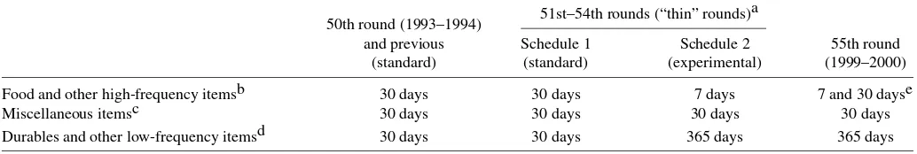
Table 1. Recall periods by round and item category
51st–54th rounds (“thin” rounds)a 50th round (1993–1994)
and previous Schedule 1 Schedule 2 55th round
(standard) (standard) (experimental) (1999–2000)
Food and other high-frequency itemsb 30 days 30 days 7 days 7 and 30 dayse
Miscellaneous itemsc 30 days 30 days 30 days 30 days
Durables and other low-frequency itemsd 30 days 30 days 365 days 365 days
aOnly one of the two schedule types was randomly assigned to each sampled household. bIncludes food, beverages, tobacco, and intoxicants.
cIncludes fuel and light, miscellaneous goods and services, rents and consumer taxes, and certain medical expenses. dIncludes footwear and clothing, durables, education, and institutional medical expenses.
eEach respondent was asked to report expenditure with both recall periods, and the responses were recorded into two parallel columns, printed next to each other in the questionnaire.
1993–1994 survey (rounds 51–54). Even if the thin rounds were not specifically designed for poverty monitoring—with doubts remaining as to the comparability of their sampling frames— each wave included an expenditure questionnaire as detailed as those adopted in the larger quinquennial rounds. In each thin round, the NSSO randomly assigned to all households in a given primary stage unit one of two questionnaire types. The first questionnaire type (Schedule 1) was the standard one, with a 30-day recall period for all items. The second type (Sched-ule 2) included instead a 7-day recall for food, beverages, and a few other items generally bought frequently, and a 365-day recall for durables, clothing, footwear, and some other low-frequency purchases. Even in Schedule 2, however, the 30-day recall was maintained for a list of items that included fuel and light, miscellaneous goods and services, rents and consumer taxes, and certain medical expenses. Table 1 summarizes the recall period used for each item category in all NSS rounds rel-evant for this article, that is, rounds 50–55.
Because the schedule type was assigned completely at ran-dom, any systematic difference in estimates between the two subsamples can be attributed to the different questionnaires as-signed to each. Consistent with previous findings in the survey literature, the results of the thin rounds showed significantly higher reported expenditure in food when the short 7-day re-call period of Schedule 2 was used rather than the standard 30-day recall of Schedule 1. For most durables, the longer (1 year) recall period of Schedule 2 led instead to lower mean expenditure than the standard 30-day recall (Sen 2000; Deaton 2001). Overall, given the large fraction of the budget spent on average in food, the net effect in all rounds and in both sectors was a larger estimate of total per capita expenditure (pcehereinafter) when the experimental Schedule 2 was used. Table 2 contains summary statistics calculated from the thin rounds. The figures were calculated using only the major In-dian states, which account for more than 95% of the total popu-lation: Andhra Pradesh, Assam, Bihar, Gujarat, Haryana (urban sector only), Jammu and Kashmir, Karnataka, Kerala, Madhya Pradesh, Maharashtra, Orissa, Punjab, Rajasthan, Tamil Nadu, Uttar Pradesh, West Bengal, and Delhi. In all surveys and in both sectors, average total pce was 10–20% higher for households in the experimental group. In all but one case, the differences were significant even using a 1% level. The only ex-ception was the urban sector in the 54th round, where the null was rejected using a 5% level. Row 6 shows that, keeping the
poverty line constant, one can “achieve” a 50% drop in poverty simply by changing the survey methodology.
Several findings emerge from the figures in rows 3–5, which refer to expenditures in those items for which a 30-day recall was maintained in both schedule types (“30-day items” here-inafter). First, mean expenditure in 30-day items differed much less between the two schedules than mean totalpce, as the ra-tio of means ranged from .93 to 1.09. In all but two cases the differences were not significant at standard levels. The two ex-ceptions were the rural sector in round 51 and the urban sec-tor in round 52, but even in these cases the null of equality of means cannot be rejected using a 1% significance level. Note also that even in these smaller surveys the sample sizes were considerable, so that the tests of equality of means have large power even when the alternative is close to the null. Overall, the evidence suggests that expenditure reports on 30-day items were only marginally affected by the different reports for food and durables in the two schedule types. Note also that expen-diture in 30-day items is a good predictor of totalpce, because it accounts for a large share of total budget. A quartic polyno-mial of (log)pcein 30-day items explains 50–60% of the total variation in (log)pcein rural areas and about 70–80% in urban areas. These two observations are important for the implemen-tation of our methodology, because they provide some prelim-inary evidence in support of using expenditure in 30-day items as a proxy variable in calculating comparable poverty estimates for the NSS round 55. But a close examination of the figures in row 3 reveals that in the rural sector mean expenditure in 30-day items was systematically higher (even if only slightly) when computed using 30-day recall data, with the opposite pat-tern seen in urban areas. This empirical regularity is likely re-lated to differences in consumption patterns and in household characteristics between the two sectors. Indeed, the survey lit-erature shows that the cognitive processes adopted to remember expenditure in a given item are associated with the characteris-tics of both the item and the respondent (see part II of Deaton and Grosh 2000). This suggests that it might be important to in-clude household characteristics among the auxiliary variables. Many of the household characteristics reported in the NSS, in-cluding household size, education, and land holdings, should also be useful predictors, and their reports are unlikely to be affected by changes in the recall periods adopted in an expen-diture survey.
318
Jour
nal
of
Business
&
Economic
Statistics
,
J
uly
2007
Table 2. Summary statistics, Indian National Sample Survey, rounds 51–54
NSS 51 NSS 52 NSS 53 NSS 54
(July 1994–June 1995) (July 1995–June 1996) (January–December 1997) (January–June 1998)
Rural Urban Rural Urban Rural Urban Rural Urban
Schedule (questionnaire type)a S1 S2 S1 S2 S1 S2 S1 S2 S1 S2 S1 S2 S1 S2 S1 S2
Sample size (no. 0 households) 13,606 13,415 9,283 9,214 12,253 12,047 8,870 8,749 12,313 9,214 16,418 10,555 8,676 8,545 2,946 2,911
Mean totalpce 273.4 310.5 462 546 279 328 495 560 294 328 469 547.4 266 316 457 521
(13.2) (3.5) (18.8) (20.1) (3.9) (3.4) (10.8) (7.5) (4.59) (4.53) (7.55) (8.50) (3.0) (2.8) (14.4) (21.4)
Ratio S2/S1 1.14 1.18 1.18 1.13 1.12 1.17 1.19 1.14
t-ratio (H0:S1=S2) 2.73 3.06 9.53 4.93 5.29 6.92 12.37 2.46
Meanpcein 30-day items 54.4 50.8 131.4 133.4 57.9 56.6 130.4 138.0 61.9 58.9 133.1 139.7 58.0 57.3 131.8 143.2 (1.5) (.8) (7.8) (7.6) (2.5) (1.1) (2.3) (2.8) (1.12) (1.31) (3.61) (3.37) (.8) (.8) (4.7) (17.8)
Ratio S2/S1 0.93 1.02 .98 1.06 .95 1.05 .99 1.09
t-ratio (H0:S1=S2) 2.12 .18 .48 2.10 1.74 1.34 .56 .62
Mean budget share 20.1 16.0 26.3 21.7 20.3 16.4 26.1 22.4 21.1 17.3 27.3 23.4 21.6 17.4 28.3 23.0 of 30-day itemsb (.22) (.17) (.40) (.34) (.16) (.14) (.17) (.18) (.23) (.22) (.21) (.21) (.14) (.12) (.39) (.33) R2OLS regression of (ln) total
pceon (ln)pcein 30-day itemsc .615 .533 .760 .787 .567 .585 .703 .742 .606 .592 .721 .743 .612 .606 .732 .761
Head count poverty ratio 41.8 22.7 36.3 18.5 38.2 18.4 30.7 15.4 35.7 21.1 33.1 17.5 41.8 22.4 35.3 21.3
Source: Author’s computations from the NSS. Robust standard errors are in parentheses. All values are in 1993–1994 rupees. The deflators are state-specific CPIIW for urban sector and CPIAL for rural sector. For NSS 54, we use sector-specific deflators. Only the major Indian states are included. All statistics are weighted using inflation factors. The poverty counts are the proportion of individuals living in households where per capita expenditure (pce) is below the poverty line. The real poverty lines are the official ones for all India published by the Planning Commission for 1993–1994 (Rs 205.7 for the rural sector, and Rs 283.4 for the urban sector).
aS1 is the standard questionnaire, with a 30-day reference period for all items. S2 is the experimental questionnaire (see Table 1 for details). bThe mean budget shares are averages of household-specific ratios between expenditure in 30-day items and total expenditure.
cTheR2is calculated from a regression of (log) total monthlypceon a polynomial of degree four of (log) monthlypcein 30-day items.
2.2 The 55th Round
The poverty estimates resulting from the four thin rounds did not help in reaching a consensus on poverty trends in India dur-ing the 1990s. In fact, the rapid GDP growth measured in the National Accounts was not reflected by poverty declines. The figures in row 6 of Table 2 show no apparent trend in poverty reduction during the period, irrespective of the schedule format. However, the thin rounds were not specifically designed as ex-penditure surveys. The relatively small samples, coupled with the choice of sampling frames more suited to the different main purposes of these surveys, caused many observers to view these poverty figures with some suspicion and to wait for the next quinquennial expenditure survey—the 55th wave of the NSS, which was completed between July 1999 and June 2000.
But the questionnaire format adopted in the 55th round was different from any other used in previous NSS surveys, com-bining both sets of recall periods used in the thin rounds (see Table 1). The new questionnaire asked all households to re-port expenditure in food and other frequently purchased items with both a 30-day and a 7-day recall, and adopted a 365-day recall for durables and other infrequent purchases. As in the thin rounds, a 30-day recall was maintained for the miscella-neous items with intermediate purchase frequency. Of the two sets of reports for high-frequency purchases, only the 30-day recall data were used by the Indian Planning Commission to calculate the official poverty counts. The results showed an impressive reduction in poverty in comparison to the early 1990s; in rural areas the head counts dropped from 37.2% in 1993–1994 to 27.1% 6 years later, whereas in urban areas the head counts dropped from 32.6% to 23.6% in the same period. But the changes in the questionnaire cast serious doubts on the comparability of the more recent figures with previous poverty estimates, especially when considering the results of the thin experimental rounds.
On the one hand, the thin rounds showed that reports on durables are on average lower when a 1-year recall period is used, so that the new questionnaire would overstate poverty. At the same time, more respondents reported some expenditure in durables, with the result that the corresponding distribution is much more spread out when the shorter recall period is used. Keeping the average report constant, this would cause the op-posite result of lower poverty estimates when the new ques-tionnaire is used. The two conflicting effects combine with the fact that durables typically account for a small share of the total budget, especially among poor households, making it unlikely that important comparability issues arise as a consequence. On the other hand, the new questionnaire recorded the two sepa-rate reports on food expenditure in two parallel columns printed next to one another. Thus this format could be expected to have prompted the respondents (or the interviewers) to reconcile the two different reports. So consumption of food reported with the traditional 30-day recall period would be disproportionately high (because the respondent would tend to avoid large discrep-ancies with the 7-day reports, which are typically higher) and/or the corresponding reports based on a 7-day recall would be disproportionately low (by a symmetric argument). The plau-sibility of this argument is strengthened by the fact that in the 55th round, averagepcein food as estimated with a 7-day recall
exceeded the corresponding figure calculated using the 30-day recall by about 6%, whereas in all of the thin rounds the gap was consistently above 30%. Because for most Indian house-holds food accounts for a very large share of the total budget, these arguments lead to the expectation that the unadjusted (of-ficial) figures overstate total expenditure, and thus understate poverty. Consequently, a methodology to estimate poverty rates comparable with previous approaches is needed. The next sec-tion describes the general econometric problem and explains how the specific empirical application (which we develop fully in Sec. 4) fits into the general framework.
3. THE MODEL AND THE ESTIMATOR
The population sampled using a revised methodology is referred to as the target population, and the one sampled us-ing a standard questionnaire as theauxiliarypopulation. Target and auxiliary surveys are defined analogously. In the empiri-cal application, NSS round 55 is the target survey, whereas we use different previous rounds as auxiliary surveys. Let Dbe a binary variable equal to 1 when an observation is drawn from the target population. Throughout the article, bold type denotes vectors and matrices and the superscript “′” indicates transpo-sition. All vectors are defined in column form.
The researcher is interested in estimating a parameterφ0in a target population, whereφ0satisfies the following population moment condition:
E[ng(y;φ0)|D=1] =0, (1) whereg(·)is a moment function,nis household size, andyis the main variable of interest as measured in a standard question-naire. In poverty or inequality measurement, ytypically mea-sures expenditure or income per head. The population moment condition (1) refers explicitly to the common situation in which the parameter of interest is defined in terms of individuals but data are sampled at the household level. If the sampling unit is the same as the unit in terms of which φ0 is defined, then all of the results that follow can be obtained as a straight-forward special case with n=1. In (1) we abstract from is-sues of intrahousehold allocation of resources, so that each individual within a household is treated equally. (See Deaton 1997, chap. 4, for an overview of the issues involved in wel-fare evaluation when household scale economies and equiv-alence scales are taken into account.) The moment condition (1) encompasses a broad set of commonly used poverty and inequality measures. (For an introduction to the theory and practice of poverty measurement, see Deaton 1997, chap. 3, or Ravallion 1992.) For example, ifφ0represents a Foster–Greer– Thorbecke poverty index and z is a fixed poverty line, then g(y;φ0)=1(y<z)(1−zy)α−φ0,whereα≥0,and1(E)is an indicator equal to 1 when eventEis true. Whenα=0,the index becomes the head count poverty ratio, whereasα=1 character-izes the poverty gap ratio. A higher parameterαindicates that large poverty gaps (1−y/z)are given a larger weight in the calculation, so that the poverty index becomes more sensitive to the distribution ofyamong the poor. Equation (1) also iden-tifies well-known inequality measures, such as the Variance of the Logarithms, ifg(y;φ0)= [(lny−φ02)2−φ01 lny−φ02]′, where φ0= [φ01 φ02]′, or the Theil index, withg(y;φ0)=
[φy02log y
φ02−φ01 y−φ02]
′.
320 Journal of Business & Economic Statistics, July 2007
3.1 Identification
Estimation of the parameter φ0 through the sample analog of (1) is clearly infeasible if the target survey does not include data on y. This is precisely the case if the survey question-naire changed in such a way that the respondents’ reports are no longer comparable with those from previous surveys, so that the researcher observes only a different variable, y, but not˜ y. In our empirical setting,yis total expenditure per head when a 30-day recall is used for all items, and y˜ is the expenditure observed when a revised questionnaire is adopted.
Let v denote a set of auxiliary variables, as recorded by a standard methodology, and letv denote the same variables as measured using a revised methodology. The set v will in-clude variables that can be used as proxies for the unob-servedy. Each observation is then characterized by the set of variables(y,y˜,v,v,D),but the econometrician observes only either(y,v),whenD=0, or(y˜,v),ifD=1. This makes clear that the parameter φ0 in (1) is not identified by the sampling process without further assumptions. The following proposition formally describes the fundamental conditions for identification that we assume throughout the article.
Proposition 1. Suppose that there exist a set of auxiliary variables, v, that include household size nand are distributed according todP(v), and assume that the following conditions hold: (A1)dP(v|D=1)=dP(v|D=1)a.s.; (A2)E[g(y;φ0)| v,D = 1] = E[g(y;φ0)|v,D = 0] a.s.; (A3) dP(v|D = 1) is absolutely continuous with respect to dP(v|D=0), and (A4) supp(v|D=1)⊆supp(v|D=0). Then φ0 satisfies the following modified population moment condition:
EnR(v)g(y;φ0)|D=0
=0, (2) whereR(v)is thereweighting function, defined as
R(v)=dP(v|D=1) dP(v|D=0)=
P(D=1|v)P(D=0)
P(D=0|v)P(D=1). (3) Moreover,R(v)is nonparametrically identified by the sampling process.
For the proof see Appendix A.
The last two assumptions, (A3) and (A4), ensure that the reweighting functionR(v)exists and is bounded for each value of v. [Note that even if (A4) does not hold, one can still es-timate bounds for the parameter of interest, treating observa-tions with v outside the common support as missing values, using the setting described in Horowitz and Manski 1995.] Assumption (A1) requires the existence of a set of proxy vari-ables v whose marginal distribution is identified by the sam-pling process in both the auxiliary and target populations. In other words, v should include variables whose distribution of reports is left unaffected by the change in survey design (note, however, that we do not require that v=v). Variables that satisfy (A1) are likely to be available in most empir-ical settings, as questionnaire revisions generally leave sev-eral questions unchanged. In our empirical application, sevsev-eral household characteristics—such as household size, education, or main economic activity—should be good candidates for in-clusion inv. Similarly, (A1) may be satisfied by reported ex-penditure in items for which the 30-day recall was retained in
all questionnaire types. Assumption (A2) requires that the con-ditional expectation of the functiong(y;φ0)is the same in the target and the auxiliary surveys. This is clearly a crucial and substantive assumption whose credibility depends on the empir-ical context and should always be carefully scrutinized. When φ0is a poverty count, (A2) amounts to assuming that the frac-tion of households to be counted as poor condifrac-tional onv re-mains constant across the two surveys. In Section 4 we devote considerable space to probe the plausibility of both (A1) and (A2) in our specific empirical setting.
The reweighting functionR(v)in (3) transforms the condi-tional expectation ofE[ng(y;φ0)|v]from the auxiliary survey into the unconditional expectation in the target survey, down-weighting (up-down-weighting) households whose auxiliary variables have a relatively high (low) density in the auxiliary survey. The conditional probability,P(D=1|v), in (3) can be interpreted as the probability that a household belongs to the target population conditional on observingv, if the household is sampled from a population that encompasses both the target and auxiliary pop-ulations. The other probabilities are defined accordingly. Note that the functionR(v)is identified by the sampling process even if the researcher only observesvˆ=Dv+(1−D)v. Indeed, in Appendix A we prove that the assumptions of Proposition 1 are sufficient to ensure thatP(D=1|ˆv)=P(D=1|v)a.s.
This form ofinverse probability weighting (IPW) has been used extensively in several settings in statistics and economet-rics. (For a textbook treatment of IPW, see Wooldridge 2001.) Horvitz and Thompson (1952) introduced weighing to account for the nonconstant probability of selection of different observa-tions within a sample (see also Wooldridge 2002a). Several con-tributions in the program evaluation literature use IPW-based estimators for the estimation of mean treatment effects, under the assumption that thepropensity score—that is, the probabil-ity that an individual participates to a program conditional on observed covariates—is the same for treated and untreated in-dividuals (see, e.g., Hahn 1998; Heckman, Ichimura, and Todd 1998; Hirano, Imbens, and Ridder 2003; Abadie 2005). Several authors have used IPW for estimation with missing data, un-der the assumption that the probability of an observation being missing depends only on some observed covariates (see, e.g., Robins, Rotnitzky, and Zhao 1994, 1995; Wooldridge 2002b). Chen, Hong, and Tarozzi (2005b) studied IPW estimators in nonlinear models of nonclassical measurement error when aux-iliary data are available.
In some cases, a researcher may be interested in recover-ing an estimate of the whole distribution of a variabley(e.g., income or expenditure per head) that is comparable with es-timates obtained before a questionnaire change took place. It is relatively straightforward to describe sufficient conditions analogous to those in Proposition 1 for identifying the density f(y|D=1). Clearly,f(y|D=1)would also identify poverty and inequality measures based ony. As in moment condition (1), we proceed under the assumption that the object of interest is the density of aper capitaquantityy, but the data are collected at thehouseholdlevel. If everyone within the household is as-sumed to be treated equally, then the individual-based popula-tion density ofy, denoted byfn(y|D=1), is described by the following expression:
fn(y|D=1)=
E[nf(y|n,D=1)] E[n|D=1] ,
wheref(y|n,D=1)is the density defined overhouseholds[it is easy to check thatfn(y|D=1)actually integrates to 1]. The following proposition formalizes conditions for identification.
Proposition 2. Suppose that there exist a set of auxiliary variables,v, including household sizen, distributed according todP(v), such that (A1), (A3), and (A4) hold. Letv−nbe a vec-tor of observed variables including all of the variables inv ex-ceptn. Suppose also that (A2b)f(y|v,D=1)=f(y|v,D=0). Then
f(y|n,D=1)=f(y|n,D=0)E[R(v−n)|y,n,D=0], (4) where the reweighting function is now defined as
R(v−n)=
P(D=1|v)P(D=0|n) P(D=0|v)P(D=1|n). For the proof see Appendix A.
We do not proceed to analyze the estimation of (4), because we are interested mainly in estimating the parameters identified by a moment condition such as that described in (1). (For an example of reweighting in the context of density estimation see DiNardo, Fortin and Lemieux 1996.)
3.2 Estimation
The modified moment condition (2) suggests that the para-meter of interest, φ0, can be estimated using a two-step pro-cedure. In the first step, the unknown probabilities P(D= 1|v) and P(D = 0) are estimated [indeed, the estimation may be further simplified noting that φ0 is identified even if P(D=0)/P(D=1)is dropped from the modified moment con-dition (2)]. In the second step,φˆ0is calculated as the solution of the sample analog of (2), after replacingR(v)with its estimate from the first step. In what follows, we proceed assuming that the sample is drawn from a “superpopulation” that encompasses both the target and the auxiliary population. ThenP(D=0) de-notes the proportion of households belonging to the auxiliary population, whereasP(D=1|v)represents the probability that a household with covariatesvsampled at random from the su-perpopulation belongs to the target population. We emphasize that both probabilities refer to the distribution of households, not individuals, and so must be estimated without inflating ob-servations by household size.
The unconditional probability P(D=0), which we denote by θ00, can be easily estimated as the fraction of households in the sample that belongs to the auxiliary population. For es-timating P(D=1|v), we assume that the conditional proba-bility is correctly described by a known parametric model, so thatP(D=1|v)=P(D=1|v;θ10), whereθ10is a vector of pa-rameters estimated with maximum likelihood. In the empiri-cal application, we model the conditional probability using a logit model. An analogous strategy was adopted by Wooldridge (2002b), Robins et al. (1995), Abadie (2005). The latter also analyzes nonparametric first-step estimators, as done by Hahn (1998), Hirano et al. (2003), or Chen et al. (2005b). A flexible functional form can be achieved using polynomials, and in any case we are interested only in obtaining good predictions for the conditional probabilities, and the parameters estimated in the binary variable model will be of little or no intrinsic interest. Moreover, it is well known that the choice of functional form
in a binary dependent variable model rarely has important con-sequences for the predicted probabilities (see, e.g., Amemiya 1985, chap. 9).
If the observations are a simple random sample, then stan-dard errors can be estimated using stanstan-dard asymptotic the-ory for two-step method-of-moments estimators (see Newey and McFadden 1994). But virtually all widely used household surveys—including the Indian NSS, the World Bank’s LSMS, the CPS and the PSID in the United States, or the Demo-graphic and Health Surveys—adopt a stratified and clustered design, making the assumption of iid observations untenable. (For an overview of the issues involved in estimation and infer-ence in multistage surveys see Deaton 1997, chap. 1.) In strat-ified and clustered surveys, the population is first divided into a fixed number ofstrata, usually defined following geographi-cal and/or socioeconomic criteria. Then a predetermined num-ber ofclusters(typically villages or urban blocks) are sampled independently from each stratum. Finally, households are se-lected independently within each cluster or, as in the NSS, from separate second-stage strata created within clusters. The use of stratification in survey design typically leads to lower standard errors, because, by construction, all possible samples become more similar to each other as a fixed proportion of observations are selected from different areas. Instead, clustering frequently leads to standard errors that are considerablyhigherthan those calculated assuming simple random sampling. This is a conse-quence of the positive correlation that is common for variables recorded in the same cluster. In most cases, the net effect of clustering and stratification is anincreasein standard errors, so that ignoring the multistage design of a survey can lead to se-riously misleading inference. Bhattacharya (2005) showed that this is indeed the case when one calculates standard errors for inequality measures in a given cross-section of the Indian NSS. In addition, because in most surveys the sampling scheme is such that the ex ante probability of selection is not the same for each households, consistent estimation of population parame-ters requires the use of sampling weights.
We estimate standard errors that take into account the presence of a complex survey design, and we derive the as-ymptotic results letting the total number of clusters grow to infinity, keeping both the number of households selected in a cluster and the proportion of clusters selected in each stra-tum constant. This setting is appropriate for our purposes, be-cause in the NSS the number of clusters is much higher than the number of households selected per cluster. Because we use observations sampled from two different databases, we need to be explicit about how the sampling from the two popula-tions is done. Here we assume that the first-stage strata are the same across the two subpopulations. Related results have been given by Bhattacharya (2005), who studied asymptotic prop-erties of generalized method-of-moments (GMM) estimators in presence of multistage surveys, in the standard situation in which all observations belong to the same population.
Letβ0= [φ0 θ10′θ00]′ denote the vector containing the true value of the parameters to be estimated (including those esti-mated in the first step), and letg(y;v,D;β0)denote the set of moments identifying all such parameters. These moments also include the scores corresponding to the conditional likelihood ofDas a function ofθ10.
322 Journal of Business & Economic Statistics, July 2007
Suppose that the population is divided intoS strata and that stratum scontains a mass ofCs clusters, indexed by c. Each cluster contains M(s,c)households, and householdh hasnsch members. Then the population moment condition can be writ-ten as
where the expectation is taken with respect to the distribution of clusters in stratums. In the first sampling stage,ns clusters are selected from thesth stratum. In the second stage,msc house-holds are selected from clustercbelonging to stratum s. The same sampling scheme is repeated independently in each stra-tum. Thus the sample analog of (5) is
0= weight. Asymptotic properties can be derived rewriting (6) as the average ofnindependent cluster-specific terms, wherenis the total number of sampled clusters. So, reindexing clusters byi, (6) becomes
In Appendix A we describe sufficient conditions for consis-tency and asymptotic normality of the estimatorβˆ. In particular, such conditions lead to the following.
Proposition 3. If assumptions A0–A8 described in Appen-dix A hold, then
√
n(βˆ−β0)→d N(0,Ŵ−1W(Ŵ−1)′), (8) where→d indicates convergence in distribution and
Ŵ=plim1
For the proof see Appendix A.
Lettinggd indicate thedth row of the vectorg(·)andβl
in-Appendix B describes the appropriate moment conditions that are relevant for our empirical application, whereφ0 is a head count ratio andP(D=1|v)follows a logistic distribution.
3.3 A Small Monte Carlo Simulation
In this section we perform a small Monte Carlo simulation to study the performance of the estimator in small samples or when the parametric model for the propensity score is misspec-ified. We also compare its performance with that of alternative estimators. For simplicity, in the Monte Carlo simulation we abstract from the presence of sampling weights and multistage survey design.
To consider a realistic data-generating process (DGP), we construct a DGP with parameters mimicking those estimated using actual data from the rural sector of the 50th and 55th rounds of the NSS. We proceed as follows. First, we assume that a univariate auxiliary variablevis distributed normally with mean and standard deviation equal to those of the logarithm of pcein 30-day items in a pooled sample that includes observa-tions from both surveys. This leads to
f(v)∼N(4.11, .5041). (11) Second, we assume that the relation between the main variable of interest y and the auxiliary variable v is described by the model
P(y<z|v)=G(.882+.16v−.141v2+.0073v3), (12) whereG(·)is the logistic distribution and the parameters have been estimated using the data from the 50th round, and setting the poverty line equal to its official value in 1993–1994 (i.e., z=5.326). Equation (12) implies thatycan be written as
y=4.444−.16v+.141v2−.0073v3+ǫ, (13) whereǫ has a logistic distribution (with mean 0 and variance π2/2) and the intercept is equal to the difference between the poverty line and the constant in the logit model (12). As a final step, we assume that the conditional probabilityP(D=1|v)is described by the logit model
P(D=1|v)=G(1.15−1.43v+.39v2−.029v3), (14) where we have estimated the parameters from the pooled sam-ple, withD=1 for observations from the 55th round.
We consider the estimation of two separate parameters:φ01= P(y<5.326|D=1), corresponding to a poverty ratio in the tar-get population, with the poverty line set at the official level for rural India, andφ02=E(y|D=1), the mean value of the vari-able of interestyin the target population. Both parameters could be trivially calculated using their respective sample analog, but we assume thatyis observed only if D=0. The true values of both parameters in either the target or the auxiliary popula-tion can be recovered by numerical integrapopula-tion making use of the assumptions embodied in (11), (12), and (14). Appendix C contains details of the calculation of the true values of the pa-rameters and of the procedure used to generate each draw from the DGP.
We analyze the performance of three different estimators. The first of these is the IPW estimator described in Section 3.2, and the second is based on a conditional expectation projection
(CEP) argument. Using the law of iterated expectations, both parameters can be rewritten as
φ0i =
v
E(qi(y)|v)f(v|D=1)dv,
whereq1(y)=1(y<5.326)andq2(y)=y. Hence each para-meter can be estimated averaging the projectionEˆ(qi(y)|v),i= 1,2, over observations from the target sample, where the pro-jection is calculated in a first step from the auxiliary sam-ple. This estimator is analogous to the CEP–GMM estimator considered by Chen et al. (2005b) and will be root-n consis-tent under appropriate regularity conditions. The third estima-tor is a “naive” estimaestima-tor where φi,i=1,2, is calculated by simply replacingyin the target survey with a predicted value
ˆ
y=E(y|v), then using the complete-data estimator of each pa-rameter of interest. The coefficients for the construction of the predicted valuesyˆare estimated from the auxiliary sample, us-ing a simple ordinary least squares (OLS) regression. Clearly, the second and third estimators of θ02 are identical, as long as they both make use of the same first-step projection. In contrast, the naive estimator will not in general be consistent for φ01; in fact, by construction, it will consistently estimate P(E(y|v) <5.326|D=1), which is in general different from P(y<5.326|D=1). Indeed, because in our simulations the “poverty line” is below the mode of the distribution, we should expect the naive estimator tounderstate poverty, because the distribution ofycan be seen as a mean-preserving spread of the distribution ofE(y|v)(see Deaton 1997, p. 151).
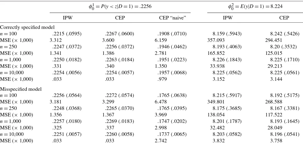
Table 3 reports the results of the simulations. We experiment with samples of size 100, 250, 1,000, and 10,000. All results are based on 1,000 replications. For each estimator we report the mean, standard deviation, and mean squared error (MSE)
of the simulations. In the top part we derive all estimates using the correct parametric functional forms identified by (11), (12), and (14). Clearly, both the IPW and CEP estimators show no sign of bias, even if for very small samples the variability of the estimates is, not surprisingly, quite large. For the calculation of poverty counts, IPW has the smallest MSE, whereas the CEP estimator performs better whenφ02is estimated. In large sam-ples, the performance of IPW and CEP are virtually identical. As expected, the “naive” estimator forφ01is systematically bi-ased downward, and the bias remains large even in very large samples. In the bottom part of the table we repeat the simula-tions but use misspecified models in all of the first-step esti-mates. In particular, in all cases where the DGP assumes the presence of a polynomial of degree 3 inv, we estimate predic-tions entering vlinearly. The results show that both IPW and CEP perform remarkably well even when the first step is mis-specified. In small samples, a misspecified first-step even leads tolowerMSE, probably because using a polynomial in the first step, even if justified by the DGP, leads to larger variability. Note instead that the performance of the naive estimator forφ10 becomes even worse. This is likely because using a linear func-tion ofvin the first step reduces the explained sum of squares ofy, leading to further underestimation of the poverty count.
In the program evaluation literature, IPW estimators have been shown to perform relatively poorly in terms of MSE with respect to matching estimators (Frölich 2004). However, the poor performance of IPW estimators is usually particularly strong when the distribution of the conditioning variables in the propensity score differs significantly between the treatment and control units. In our context, these large differences are unlikely to be of concern. In this article the propensity score represents the probability that an observation belongs to the target survey,
Table 3. Results of Monte Carlo simulation
φ01=P(y<z|D=1)=.2256 φ02=E(y|D=1)=8.224
IPW CEP CEP “naive” IPW CEP
Correctly specified model
n=100 .2215(.0595) .2267(.0600) .1908(.0710) 8.159(.5943) 8.242(.5426)
MSE (×1,000) 3.312 3.600 6.159 357.093 294.451
n=250 .2247(.0372) .2256(.0372) .1946(.0462) 8.193(.4063) 8.20(.3532)
MSE (×1,000) 1.341 1.386 2.781 165.852 125.015
n=1,000 .2250(.0182) .2263(.0184) .1951(.0223) 8.226(.1843) 8.225(.1710)
MSE (×1,000) .331 .340 1.350 33.938 29.213
n=10,000 .2254(.0056) .2254(.0057) .1957(.0068) 8.225(.0562) 8.225(.0561)
MSE (×1,000) .033 .033 .979 3.152 3.144
Misspecified model
n=100 .2256(.0564) .2272(.0574) .1765(.0638) 8.215(.5917) 8.192(.5175)
MSE (×1,000) 3.181 3.299 6.478 349.801 268.588
n=250 .2248(.0368) .2265(.0370) .1765(.0395) 8.175(.3685) 8.167(.3381)
MSE (×1,000) 1.356 1.367 3.969 138.054 117.522
n=1,000 .2257(.0180) .2269(.0183) .1747(.0202) 8.201(.1787) 8.193(.1645)
MSE (×1,000) .325 .337 2.998 32.482 28.049
n=10,000 .2251(.0057) .2260(.0058) .1737(.0065) 8.203(.0582) 8.196(.0541)
MSE (×1,000) .033 .033 2.742 3.832 3.758
NOTE: All results are based on 1,000 replications. For details on the DGP and the estimators, see Section 3.3 and Appendix C. We analyze the performance of three different estimators. IPW is the IPW estimator described in Section 3.2. The estimator in column 2 is calculated as an average over the target sample of the predicted value for the probability of being poor conditional onv. The results in columns 3 and 5 use the “naive” sample analogs of each parameter of interest, calculated replacing the true value ofywith its prediction from a first-stage OLS regression. The figures listed to the right of the sample sizes are means and (in parentheses) standard deviations of the estimates calculated over the 1,000 replications.
324 Journal of Business & Economic Statistics, July 2007
conditional on a set of proxy variables, whereas the roles of the treatment and control groups are filled by the target and aux-iliary samples. The validity of the identifying assumptions un-derlying our estimation procedure will typically require using auxiliary and target surveys relatively close in time to one an-other (see also Sec. 4), so that the two subsamples usually will be well balanced.
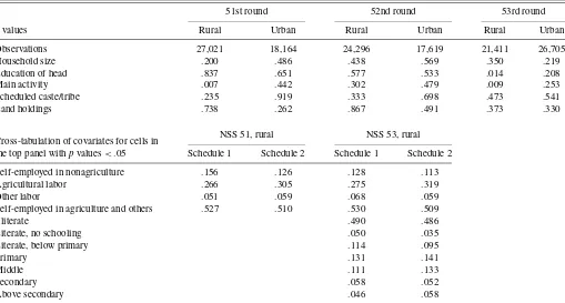
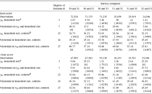
4. AN APPLICATION TO POVERTY IN INDIA In Section 2 we described how the expenditure schedule adopted in the 1999–2000 round of the Indian NSS included a set of recall periods different from all previously adopted ones (see Table 1), while leaving several sections of the ques-tionnaire unchanged. In particular, expenditure data on a list of miscellaneous items were collected using a 30-day recall common to all NSS rounds, and information on a set of house-hold characteristics was recorded in a consistent fashion across all different surveys. Hence, under the assumptions described in Section 3, all of these covariates can be used as auxiliary variables to estimate poverty counts for 1999–2000 that are comparable with those from previous years, by applying the methodology described in Section 3.2. As auxiliary databases, we use NSS surveys completed in previous years with a stan-dard questionnaire, that is, the 50th round and the component of the thin rounds from the 51st to the 53rd rounds that used a uniform 30-day recall. We do not use data from the 54th round, because this survey was carried out over a 6-month period in-stead of a whole year as for all other surveys, so that seasonality issues might cause comparability problems.
In our choice of auxiliary variables, we are limited by the fact that several household characteristics are recorded only in the quinquennial surveys, whereas others are recorded differ-ently across different rounds. For instance, the quinquennial rounds include more information than the thin rounds on hous-ing characteristics and the way in which such information is coded differs across surveys. Similarly, in 1999–2000 the main “industry” that employs the household is coded differently from previous rounds. In other words, the inclusion of several proxies as auxiliary variables would probably create further compara-bility problems across surveys rather than solving the one cen-tral to our study. Hence we focus on a limited set of variables, including household size and categorical variables for the main economic activity of the household, land holdings, education of the head, and whether the household belongs to a scheduled caste or tribe. In fact, there are some differences in coding even among these categorical variables, but different coding schemes are nested, so that it is easy to make reports comparable across surveys.
Before proceeding with the actual implementation of our ad-justment procedure, considering to what extent its results would be expected to be valuable in our empirical framework would be useful. In Section 4.1 we interpret the meaning of the iden-tifying assumptions (A1) and (A2) of Proposition 1 in our spe-cific application, and we discuss reasons why these assumptions could fail. Clearly, neither (A1) nor (A2) can be tested directly, because both assumptions are defined in terms of variables that are not observed. However, indirect evidence supporting their validity can be obtained by using the data collected in the thin
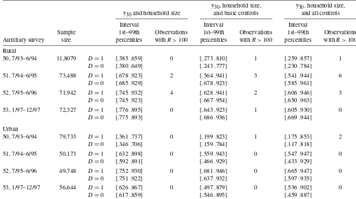
rounds, in which two different questionnaire types were as-signed at random at respondents living in different clusters. The random assignment implies that in each thin round the distrib-ution of both(y,v)(from Schedule 1) and(y˜,v)(from Sched-ule 2) are identified, where we have used the notation laid out in Section 3.1, with a tilde denoting variables measured with a revised questionnaire. We exploit this information in two differ-ent ways. First, in Section 4.2 we construct formal tests for the validity of assumptions (A1) and (A2) within the thin round, be-cause the sampling process identifies all relevant distributions. Second, in Section 4.3 we describe an experiment to evaluate the performance of our estimator. For each thin round, we can estimate a “comparable” head count using data from the subset of households who received a standard questionnaire. Then we can attempt to replicate this benchmark using data onvfrom Schedule 2 and using one of the standard surveys as an aux-iliary survey. If the conditions in Proposition 1 hold, then the benchmark and the adjusted estimates should differ only due to sampling error.
We reiterate that the investigations that we have just de-scribed can provide only indirect evidence in support of the untestable identifying assumptions necessary for calculating comparable head counts for 1999–2000. A second caveat is that the experimental questionnaire adopted in the thin rounds is not identical to that eventually adopted in 1999–2000. For this reason, the experiments do not exactly mimic the adjust-ment necessary to recover comparable head counts from the latest quinquennial round. Nonetheless, the indirect evidence presented here should provide further support as to the appro-priateness of the adjustment procedure.
4.1 Plausibility of the Identifying Assumptions
Assumption (A1) requires that the distribution of reports for the auxiliary variables in the target survey be the same as the distribution that would have been observed had no question-naire change occurred. If the questionquestion-naire revision does not affect sections in which the variables invare reported, then this assumption may appear innocuous, but there are reasons why it may be invalid. For instance, a longer list of expenditure items included in a revised questionnaire might affect reporting error for all variables, because it can increase weariness in the subject interviewed. Thus, if the many questions on food expenditure (which come first in the questionnaire) are asked using both a 7-day and a 30-day recall rather than with a single recall, then a tired respondent may be tempted to cut the rest of the interview short, reporting zero expenditure on a large number of the items that follow. Alternatively, the presence and wording of certain (modified) questions may influence the way in which the re-spondent remembers or processes information that is relevant for other (unchanged) questions. For instance, a 365-day recall for hospitalization costs may lead the respondent to remember an illness episode that took place 2 months ago, in turn leading him to remember an expenditure in drugs incurred during the last week at home—and so included in expenditure in 30-day items—but related to that hospitalization episode. The respon-dent may not have remembered the drug expenses if the survey had used a uniform 30-day recall. Note that these concerns are less likely to arise for most demographic and occupational char-acteristics of the household. These variables are usually much