Full Terms & Conditions of access and use can be found at
http://www.tandfonline.com/action/journalInformation?journalCode=ubes20
Download by: [Universitas Maritim Raja Ali Haji] Date: 13 January 2016, At: 00:38
Journal of Business & Economic Statistics
ISSN: 0735-0015 (Print) 1537-2707 (Online) Journal homepage: http://www.tandfonline.com/loi/ubes20
Semiparametric Estimation of the Optimal Reserve
Price in First-Price Auctions
Tong Li, Isabelle Perrigne & Quang Vuong
To cite this article: Tong Li, Isabelle Perrigne & Quang Vuong (2003) Semiparametric
Estimation of the Optimal Reserve Price in First-Price Auctions, Journal of Business & Economic Statistics, 21:1, 53-64, DOI: 10.1198/073500102288618757
To link to this article: http://dx.doi.org/10.1198/073500102288618757
Published online: 01 Jan 2012.
Submit your article to this journal
Article views: 51
View related articles
Semiparametric Estimation of the Optimal
Reserve Price in First-Price Auctions
Tong
Li
Department of Economics, Indiana University, Bloomington, IN 47405-5301 (toli@indiana.edu)
Isabelle
Perrigne
and Quang
Vuong
Department of Economics, University of Southern California, Los Angeles, CA 90089-0253 (perrigne@usc.edu,qvuong@usc.edu)
The optimal reserve price in the independent private value paradigm is generally expressed as a func-tional of the latent distribution of private signals, which is by nature unobserved. This feature has limi-ted the implementation of the optimal reserve price in practice. In this article, we consider rst-price auctions within the general afliated private values paradigm. We show that the seller’s expected prot can be written as a functional of the observed bid distribution. We propose a semiparametric extremum estimator for estimating consistently the optimal reserve price from observed bids. As an illustration, we consider the Outer Continental Shelf (OCS) wildcat auctions.
KEY WORDS: Afliated private value; OCS wildcat auction; Semiparametric extremum estimator.
Given the monopoly power of the seller in an auction, the economic literature has focused on how the seller can extract the largest revenue or prot. The problem of optimal auctions is to nd the auction mechanism that provides the greatest revenue or prot for the seller. This is of considerable practical value because many commodities are sold through auctions. Because any auction mechanism, such as rst-price, second-price, English, and Dutch auctions, generates the same revenue for the seller in the independent private value (IPV) paradigm with risk neutral bidders, as shown by Vickrey (1961), the problem of optimal mechanism design reduces to determining the optimal reserve price. The latter is expressed as a func-tional of the distribution of private values and its correspond-ing density function. See the work of Laffont and Maskin (1980), Harris and Raviv (1981), Myerson (1981), and Riley and Samuelson (1981).
Despite its economic importance, this result has been of little practical usefulness in empirical studies. As argued by McAfee and Vincent (1992) and Hendricks and Paarsch (1995), a major difculty in implementing the optimal reserve price is the use of unobservables such as the latent distribu-tion of private signals. Hence, very few empirical studies were attempted to assess the optimal reserve prices using eld auc-tion data. In particular, McAfee and Vincent (1992) gave an approximation of the optimal reserve price for Outer Conti-nental Shelf (OCS) auctions in the common value framework. Paarsch (1997) proposed an estimate of the optimal reserve price from English auction data relying on parametric assump-tions on the distribution of private values. Moreover, to our knowledge, the optimal reserve price has been obtained for the IPV paradigm only. This can be restrictive given its inde-pendence assumption because there are auctions in which the IPV paradigm does not apply.
In this article, we consider the afliated private values (APV) paradigm, which includes the IPV paradigm as a spe-cial case, and we propose a direct method for estimating the optimal reserve price. In particular, we characterize the opti-mal reserve price in rst-price sealed-bid auctions with
sym-metric and risk neutral bidders. The reserve price is optimal in the sense that it generates the highest expected prot for the seller in a rst-price auction. Thus we do not consider the optimality of the auction mechanism because, for instance, a second-price auction would generate a higher prot for the seller; see Milgrom and Weber (1982). With risk averse bid-ders, the optimal auction mechanism is much more complex and involves some transfer payments; see Maskin and Riley (1984). Next, we show that the seller’s expected prot can be written as a functional of the observed bid distribution. This can be used to derive the optimal reserve price from observed bids as the maximizer of this function. We then propose a semiparametric extremum estimator for estimating consistently the optimal reserve price from observed bids. Specically, the estimated optimal reserve price is obtained as a maximizer of an estimated prot function in which some unknown distributions and densities have been nonparametri-cally estimated in a rst step. Our procedure is computatio-nally simple because it does not require computation of the equilibrium strategy. It does not require a parametric speci-cation of the distribution of unobserved private values or nonparametric estimation of the latter, as in our other work (Li, Perrigne, and Vuong, 2002). We show that our estimator is consistent. In addition to being more direct and computa-tionally simpler, our estimator can converge at a faster rate than the one based on the estimation of the underlying private values distribution.
We illustrate our methodology with the U.S. gas lease auc-tions off the coast of Louisiana and Texas, which have been studied in the literature. See Porter (1995) for a survey. We focus on wildcat auctions between 1954 and 1969 because bidders in these auctions can be considered as symmetric and
©2003 American Statistical Association Journal of Business & Economic Statistics January 2003, Vol. 21, No. 1 DOI 10.1198/073500102288618757
53
the crude oil market was relatively stable during that period. It is widely recognized that the reserve price in these auctions was too low; see, for example, the work of McAfee and Vincent (1992). Our empirical ndings indicate that the opti-mal reserve price would (i) allow the federal government to extract a larger proportion of oil companies’ willingness to pay and (ii) generate a higher prot and higher revenues for the federal government despite more tracts remaining unsold. The article is organized as follows. Section 1 is devoted to the derivation of the optimal reserve price in rst-price auc-tions using observed bids. Section 2 develops our semipara-metric extremum estimator. Section 3 illustrates our method. Section 4 concludes. The Appendix collects the proofs of our propositions as well as their applications to the IPV case.
1. OPTIMAL RESERVE PRICE IN FIRST-PRICE AUCTIONS
1.1 The Private Value Model
Throughout the article we consider rst-price sealed-bid auctions within the private value paradigm. Formally, a
sin-gle and indivisible object is auctioned to n bidders who are
assumed to be risk neutral. All sealed bids are collected simul-taneously. Provided that bid is at least as high as a reserve price, the highest bidder wins the auction and pays the bid. The utility of each buyeriD11 : : : 1 nfor the object isvi. The vector4v11 : : : 1 vn5is a realization of a random vector whose n-dimensional cumulative distribution function is F 4¢5 with support 6v1 v7n. This distribution is assumed to be afliated
as dened by Milgrom and Weber (1982). Roughly, afliation means that large values for some of the components make the other components more likely to be large than small. Each bid-der knows his or her private valuevi and the distributionF 4¢5
from which v11 : : : 1 vn are jointly drawn but does not know
other bidders’ private values. We restrict our study to the case in whichF 4¢5is exchangeable in itsnarguments. This model
is known as the symmetric afliated private value model. As far as we know, despite its generality, the APV model has seldom been studied in the literature, except in experimen-tal studies by Kagel, Harstad, and Levin (1987), in empirical studies by Li, Perrigne, and Vuong (2000), and in simulation studies by Li et al. (2002).
At the Bayesian Nash equilibrium, bidder i chooses bid
bi to maximize E64viƒbi5 4Biµbi5—vi7, where BiDs4yi5,
yiDmaxj6Divj, ands4¢5 is the strictly increasing equilibrium
strategy. Assume rst that the reserve price is nonbinding. The equilibrium strategy satises the rst-order differential equa-tion
s04vi5D6viƒs4vi57fy
1—v14vi—vi5=Fy1—v14vi—vi5 (1)
for all vi 26v1 v7 subject to the boundary condition s4v5D
v, where Fy1—v14¢—¢5 denotes the conditional distribution of y1
givenv1,fy1—v14¢—¢5denotes the corresponding density, and the
index 1 refers to any bidder among the n bidders because
all bidders are ex ante identical. From Milgrom and Weber (1982), the explicit solution of (1) is
biDs4vi5Dviƒ Zvi
v
L4—vi5d1 (2)
whereL4—vi5Dexp6ƒ Rvi
fy1—v14u—u5=Fy1—v14u—u5du7.
We next introduce a binding reserve pricep0> v. The
intro-duction of a reserve price acts as a screening device for par-ticipating in the auction. The screening level is a function of
p0 such that those bidders with private signals strictly below
this level will not bid. From Milgrom and Weber (1982), it can be easily shown that the screening level in the APV model is exactly the reserve pricep0. The equilibrium strategy becomes
biDs4vi1 p05DviƒZvi
p0
L4—vi5d for vi¶p00 (3)
In particular,s4vi5given in (2) is identical tos4vi1 v5.
1.2 The Optimal Reserve Price
The choice of the reserve price constitutes an impor-tant instrument with which the seller can take advantage of monopoly power and increase prots from the auction. As far as we know, the characterization of the optimal reserve price in a rst-price sealed-bid auction within the APV paradigm has not been derived in the literature. This is the purpose of the next proposition.
Proposition 1. In a rst-price sealed-bid auction with
n¶2 bidders within the APV paradigm, the optimal reserve
pricepü
0 that maximizes the expected prot for the seller
sat-ises
p0üDv0C
Rv
pü0L4p0ü—u5Fy1—v14u—u5fv14u5du Fy
1—v14p
ü
0—p0ü5fv14p
ü
05
(4)
ifv < p0ü< v, wherev0 denotes the private value of the seller
for the auctioned object, fv14¢5is the marginal density of vi,
and Fy1—v14¢—¢5and L4¢—¢5 are as dened earlier. [Equation (4)
may have multiple roots. If this is the case, it is necessary to evaluate the expected prot at each root to determine the global maximum, as is usually advised in the theoretical liter-ature.]
The conditionv < pü
0< v arises from the characterization
of a maximum through its rst-order condition (4). It is not a primitive condition and thus calls for some comments. First, note that whatever a seller’s private value v0, the seller does not lose expected prot by only choosing a reserve price belonging to the closed interval6v1 v7. The intuition is quite simple as any reserve price larger thanvor smaller thanvwill generate the same expected prot as whenp0Dvandp0Dv, respectively. The latter arises from the boundary condition
s4v1 p05Dvfor anyp0µvso that the equilibrium strategy is identical to (2) in this case. Second, if the seller’s private value
v0 belongs to 6v1 v5, then the optimal reserve price pü
0 must
belong to 4v1 v5 as required in Proposition 1: the seller will always increase the prot by setting a reserve price slightly
larger than v because the derivative of the expected prot is
strictly positive in the neighborhood of this point. It follows thatv0< pü
0< vfor anyv026v1 v5. Third, ifv0¶v, thenpü0Dv
because the seller does not gain by setting a higher reserve price. Fourth, ifv0< v, thenpü
0Dv orpü024v1 v5depending
on the underlying distribution of private values. In particular, this implies that a nonbinding optimal reserve price, that is,
pü
0µv, impliesv0< v.
As is well known, a special case of the APV paradigm is the IPV paradigm rst considered by Vickrey (1961), wherein private values are drawn independently from a common dis-tributionF 4¢5. All other assumptions made previously for the
APV case remain valid. In the IPV paradigm, the optimal reserve price has been widely studied (Laffont and Maskin 1980; Riley and Samuelson 1981). The optimal reserve price
pü
0 in a rst-price auction solves
pü0Dv0C1ƒF 4pü05 f 4pü
05
(5)
if v < pü
0 < v. It can be easily checked that (5) follows
from (4) by noting that L4—v5 and Fy1—v14v—v5 reduce to 4F 45=F 4v55nƒ1 and Fnƒ14v5, respectively, in the IPV case.
A remarkable property of p0ü is that it does not depend on
the number of bidders as well as the auction mechanism used because of the revenue equivalence theorem.
As expected, the optimal reserve price in the APV paradigm crucially depends on the latent distribution of private sig-nals throughFy1—v14¢—¢5,fy1—v14¢—¢5andfv14¢5. [Levin and Smith
(1996) studied the optimal reserve price in the APV model without giving its expression. An interesting question is the effect of the numbernof bidders on the optimal reserve price. Their results suggest that the optimal reserve price decreases
with n in second-price auctions.] Unfortunately, these
func-tions are unknown to the analyst, which limits the application of (4) or (5) on eld data. This is a typical problem in the optimal auction literature whatever the paradigm under con-sideration. Such a difculty was mentioned by McAfee and Vincent (1992), Hendricks and Paarsch (1995), and Paarsch (1997) among others. The structural econometric approach developed by Paarsch (1992), Laffont, Ossard, and Vuong (1995), and Guerre, Perrigne, and Vuong (2000) offers econo-metric methods for estimating the latent distribution in the IPV model. More recently, Li et al. (2002) extended the structural approach to the APV model by developing a two-step proce-dure for estimating the latent distribution nonparametrically. See Perrigne and Vuong (1999) for a survey of recent devel-opments. Although this procedure can be used to determine the optimal reserve price, in this article we propose a more direct and simpler method with superior statistical properties.
1.3 A Reformulation from Observed Bids
Assume that we observe bids from a rst-price sealed-bid auction with a nonbinding reserve price. If observed bids are coming from a rst-price auction with a reserve price, the func-tion4¢5dened in the following becomes more involved; see
the IPV case of Guerre et al. (2000). Nonetheless, a similar argument can be applied to obtain a characterization of the opti-mal reserve price from the observed bid distribution. As postu-lated in the structural approach, such bids are the equilibrium
bids of the corresponding game and hence are given bybiD
s4vi5, wheres4¢5is dened by (2). Because private values are
random, bids are naturally random with ann-dimensional joint distribution G4¢5. Moreover, because s4¢5 is strictly increas-ing, we haveGB1—b14X—x5DFy1—v14sƒ14X5—sƒ14x55, whereB1D
maxj6D1bjDs4y15andGB1—b14¢—¢5denotes the conditional
distri-bution ofB1givenb1. It follows that the corresponding density
is given by gB1—b14X—x5D fy1—v14s
ƒ14X5—sƒ14x55=s04sƒ14X55.
Thus the differential equation (1) can be written as
vDbCGB1—b14b—b5 gB
1—b14b—b5
²4b50 (6)
As noted by Li et al. (2002), the function4¢5is the inverse
bidding strategysƒ14
¢5in a rst-price sealed-bid auction with
a nonbinding reserve price.
The next proposition characterizes the optimal reserve price
in terms of the observed bid distribution. Let GB
11b14¢1¢5
be the joint distribution of 4B11 b15 with density gB11b14¢1¢5
and support 6b1 b72. Let G
B1b14¢1¢5 D¡GB11b14¢1¢5=¡b1 D GB1—b14¢—¢5gb14¢5.
Proposition 2. The optimal reserve price pü0 in a
rst-price sealed-bid auction with n¶2 bidders within the APV
paradigm can be written aspü
0D4x05forbµx0µb, where
4¢5 is dened as (6) and x0 maximizes with respect to
x26b1 b7the expected prot
ç4x5DE£
v0 4B1µx5 4b1µx5
Cn6b1C44x5ƒx5å4x—b157
4B1µb15 4b1¶x5 ¤
1 (7)
where å4r—t5 Dexp4ƒRrtgB11b14u1 u5=GB1b14u1 u5du5, E6¢7
denotes the expectation with respect to 4B11 b15, and 4¢5
denotes the indicator of the event in parentheses. [The third term in (7) arises from adopting a game theoretic approach, which takes into account the dependence of bidders’ behavior on the reserve price. In contrast, a decision theoretic approach would consider the rst two terms only in (7) and would give
pü
0Dv0.]
Note that if v0 2 6v1 v5, then x0 2 4b1 b5D4s4v51 s4v55
becausex0Ds4pü05andv < pü0< vas noted before. In contrast
to Proposition 1, which requires the knowledge of the under-lying distributionsFy1—v14¢—¢5 andfv14¢5 of private signals, the
main advantage of Proposition 2 is that it expresses the opti-mal reserve price in terms of the bid distribution, which can be estimated directly from observed bids. This is the basis of our direct procedure for estimating the optimal reserve price, as presented in the next section.
2. ECONOMETRIC IMPLEMENTATION
In agreement with Section 1.3, we consider L rst-price
auctions with a nonbinding reserve price and we assume that bidders’ payoffs for each auction do not depend on bidders’ past actions to prevent dynamic considerations. As postulated in the structural approach, observed bids are assumed to obey the equilibrium strategy (2) within each auction. To simplify the presentation, we also assume that auctions are homoge-neous so that there is no need to control for heterogeneity of the auctioned objects through some vector of characteristics. Allowing for heterogeneity of the auctioned objects through a vector z2òd of characteristics is straightforward. In this
case, our methods estimate the optimal price for an arbitrary valuez0. For instance, ifzD4z11 : : : 1 zd5includes only
con-tinuous variables and z` denotes the value of z for the `th
object, it sufces to insert the term QdkD1K44zk0ƒzk`5=hz5in
(8) and (9).
Let ` index the `th auction, and let n` be the number of
bidders in the `th auction with n` ¶2. The observed bids
are8bi`1 iD11 : : : 1 n`1 `D11 : : : 1 L9. This section proposes a direct method for estimating the optimal reserve price pü
0 in
rst-price sealed-bid auctions within the APV paradigm from such observations without making parametric assumptions.
Our method relies on Proposition 2. Specically, as pü
0D 4x05, a natural estimator of pü
0 is pO0üD O4xO05, where 4O ¢5
and xO0 are estimators of 4¢5 and x0, respectively.
Regard-ing 4¢5, which is the inverse of the equilibrium strategy
s4¢5, we follow Li et al. (2002). Regardingx0, Proposition 2
indicates that, if the prot function ç4¢5 can be estimated
sufciently well, then x0 could be estimated by xO0, where
O
x0 maximizes the estimated prot function. This is the
pur-pose of the second subsection. [Alternatively, we could use the rst-order condition corresponding to the maximization
of (7) with respect to x. This would lead to
semiparamet-ric Generalized Method of Moments (GMM) estimation of
x0 (Newey 1994; Newey and MacFadden 1994; Olley and
Pakes 1995), in which the unknown distributions and densi-ties are estimated nonparametrically in a rst step. Note that such an estimation method would require estimation of the derivative04
¢5, which can be estimated only at a slower rate
than 4¢5. This method is left for future research.
Speci-cally, when x024b1 b5, which occurs if v < pü0< v, then x0
can be characterized by its rst-order condition 0DE644x5ƒ
v05GB
1b14x1 x5ƒ 4B1 µ b15 4b1 ¶ x5
04x5å4x—b
157. This
rst-order condition is obtained after some algebra by differ-entiating (7) with respect to x and usingdGB11b14x1 x5=dxD
nGB1b14x1 x5, GB1—b14x—x5gb14x5DGB1b14x1 x5, 4x5ƒxD
GB1b14x1 x5=gB11b14x1 x5, and (A.6).] Because the expected
prot ç4¢5 involves unknown functions, namely, GB1b14¢1¢5
and gB11b14¢1¢5, this leads naturally to considering
semipara-metric M-estimation, in which these distributions and densities are estimated nonparametrically in a rst step. Thus our semi-parametric M-estimator corresponds more to the terminology used by Andrews (1994) and Powell (1994) than to that used by Newey and MacFadden (1994).
2.1 Nonparametric Estimation of4¢5
Our rst step is to estimate the inverse equilibrium strategy
4¢5 from observed bids. Note that this function depends on
the numbern of bidders. To emphasize such a dependence,
we denote it by4¢—n5. Following Li et al. (2002) and Guerre et al. (2000), we use kernel estimators, although any other nonparametric estimators can be employed.
To estimate 4¢—n5, we consider only bids from auctions
with n bidders, namely, 8bi`1 i D11 : : : 1 n1 `D11 0 0 0 1 Ln9,
where Ln is the number of such auctions. Noting that
GB
1—b14¢1¢5=gB1—b14¢1¢5DGB1b14¢1¢5=gB11b14¢1¢5, it follows from
(6) that the inverse equilibrium strategy 4¢—n5 can be
estimated by 4bO —n5DbCGbB1b14b1 b5=gOB11b14b1 b5 for any
for any value4B1 b5withhG andhgsome smoothing
parame-ters called bandwidths, and K4¢5 a weight function called
kernel satisfying Assumption A2 in the Appendix. Note that
the symmetry of bidders was used by averaging overi in (8)
and (9).
As shown by Li et al. (2002, prop. A1), if Assumption A1
in the Appendix holds, then GB
1b14¢1¢5 and gB11b14¢1¢5 have
bothRCnƒ2 continuous bounded partial derivatives on any
compact subsets of 4b1 b52, where R is the differentiability
order of the joint densityf 4v11 : : : 1 vn5of private values. Let
wherecGandcgare some constants. From Stone (1982), these
bandwidths are optimal in the sense of delivering the fastest
rates of uniform convergence for estimating GB
1b14¢1¢5, gB
11b14¢1¢5, and hence the inverse equilibrium strategy4¢5. See
Lemma A.1 in the Appendix.
2.2 Semiparametric M-Estimation ofx0
As shown in Proposition 2,x0maximizes the expected prot
functionç4¢5. It is thus natural to estimate x0 by the value that maximizes an estimated prot function. This motivates our estimator as an extremum or M-estimator preceded by a nonparametric rst step. Note thatx0generally depends on the
numbernof bidders.
Proposition 2 provides an expression (7) for the expected
prot function ç4¢5. Specically, noting that 4x5ƒxD
GB1b14x1 x5=gB11b14x1 x5, (7) can be written as ç4x5 D
E6–4B11 b11 x1 gB11b1=GB1b157, where–4¢5is given by the term
in brackets in (7). This leads to considering the estimated expected prot function by averaging over bids the function
–4¢5, where GB1b1 andgB11b1 are replaced by their
nonpara-metric estimates (8) and (9), namely,
b
mated uniformly if u and hence t are too close to the upper
boundaryb. See Lemma A.1.
DenexO0n as maximizing the estimated expected protç4b ¢5
over 6bminC„1 bmaxƒ„7, where bmin is the minimum of the
bids bi`, iD11 0 0 0 1 n, `D11 0 0 0 1 Ln. More rigorously,xO0n is
dened as any value in6bminC„1 bmaxƒ„7that satises
b
ç4xO0n5¶ sup x26bminC„1bmaxƒ„7
b
ç4x5Co4151 (12)
where o415 converges to zero as Ln! ˆ. Because bç4¢5 is
piecewise continuous inx, the termo415ensures the existence of xO0n. [Because the statistical objective function4O ¢5is not
continuous, our estimator cannot be characterized by its rst-order conditions.]
Because x0n maximizes the expected prot ç4¢5, whereas
O
x0n essentially maximizes the estimated expected prot bç4¢5,
it is expected that the latter is a consistent estimator of the former. This is formally established in the next propo-sition, which relies on Lemma A.2. This lemma extends Theorem 4.1.1 of Amemiya (1985), which is fundamental for establishing the consistency of extremum estimators. Besides allowing for a discontinuous statistical objective function, our lemma allows for maximization and uniform consistency over an expanding subset. [Andrews (1995) also considered expanding subsets to trim out observations for which the esti-mated density is too close to zero. In contrast, our expand-ing subsets arise from trimmexpand-ing close to the boundaries of the compact support of the bid distribution. Alternatively, we could consider maximization of (12) over a xed compact sub-set 6a1 a7 included in4b1 b5. The interval4b1 b5 is, however, unknown, although it can be estimated by4bmin1 bmax5. More
important,x0n is not guaranteed to belong to the chosen xed compact subset. Requiringx0n26a1 a7imposes some
restric-tions on the seller’s private valuev0and the underlying
distri-butionF 4¢5.]
Proposition 3. Suppose that p0ü is the unique maximizer of the seller’s expected prot over6v1 v7and thatv < pü
0< v.
If Assumptions A1 and A2 hold withR¶n¶2, thenxO0n is a strongly consistent estimator ofx0n asLn! ˆ.
As noted earlier, there is no loss in requiring that pü
0n 2 6v1 v7. The uniqueness assumption is necessary for identica-tion, whereasv < pü
0< vis satised ifvµv0< v.
Combining Proposition 3 and the uniform consistent esti-mation of 4¢—n5 in Section 2.1 delivers a consistent
esti-mator of the optimal reserve price pü0n. The additional sub-script n emphasizes that pü
0n generally depends on n in the
APV paradigm. Specically, under the assumptions of Propo-sition 2, pOü0n D O4xO0n—n5 is a strongly consistent estimator
of pü
0n as Ln ! ˆ. The rate of convergence of pO0ün is at
best that of 4O ¢—n5, namely,L4RCnƒ25=42RC2nƒ25
n from Li et al.
(2002, prop. 2(i)). In particular, ifx0n ispLn-consistent as in Andrews (1994), our estimatorpOü
0n would be consistent at the
rateL4RCnƒ25=42RC2nƒ25
n .
As mentioned, an alternative method for estimating the optimal reserve price is rst to estimate the APV model, namely, the underlying joint density f 4¢1 : : : 1¢5, and then
to use (4), where fv14¢5 and fy1—v14¢—¢5 are replaced by
their corresponding nonparametric estimates. From Li et al.
(2002, prop. 3), the marginal density estimator fOv
14¢5
converges at the rate L4RCnƒ25=42RC2nC25
n while the
condi-tional density estimator fOy1—v14¢—¢5 converges at the rate
L4RCnƒ252=64RCnC1542RC2nƒ257
n , which is strictly slower. The latter
consistency rate is established by following the proof of Proposition 3 of Li et al. (2002) with a bandwidth rate of the form c4logLn=Ln54RCnƒ25=64RCnC1542RC2nƒ257 when
estimat-ing the bivariate densityfyv4¢1¢5, which hasRCnƒ2 contin-uous derivatives from Lemma A1(iii) in that article. Hence, the convergence rate of this alternative estimator ofpü
0n is at
best L4RCnƒ252=64RCnC1542RC2nƒ257
n , which is strictly slower than
the previous rateL4RCnƒ25=42RC2nC25
n .
3. AN ILLUSTRATION OF OCS WILDCAT AUCTIONS
It was widely recognized by economists that the reserve price used by the federal government in OCS auctions was too low (Hendricks, Porter, and Spady 1989; McAfee and Vincent 1992; Hendricks, Porter, and Wilson 1994). As argued by McAfee and Vincent (1992), however, a roadblock to apply-ing auction theory and especially to determinapply-ing the optimal reserve price is the knowledge of unobservables. This section proposes an estimate of the optimal reserve price in OCS wild-cat auctions using our semiparametric estimator within the private value paradigm. [The previous literature on OCS data used the so-called mineral rights model or (pure) common value (CV) model. In the APV model, afliation among pri-vate values can arise from an unobserved common component. See Li et al. (2000) for the formalization of such a model. The basic difference between an APV model and a common value model is the specication of a bidder’s utility, which is the bidder’s own private value when considering a private value model and the unknown common component when con-sidering a pure common value model. Consequently, the APV model does not incorporate a winner’s curse, which is present in the CV model. Although the APV model does not exclude the existence of a possible common component through the afliation of bidders’ private values, it assumes that each com-pany’s utility is idiosyncratic and related to rms’ opportunity costs and efciency. On the other hand, the CV model assumes that each company’s utility is identical whatever the rm’s opportunity costs and efciencies, which could be restrictive. It is likely that the real situation is between these two polar cases in that the utility of each bidder is a function of both common and private components.]
3.1 Data
The U.S. government began auctioning its mineral rights to offshore oil and gas off the Texas and Louisiana coasts in 1954. The auctioned tracts are usually of about 5,000 acres. The bidders are oil companies. The auction is organized as a rst-price sealed-bid auction with a reserve price of $15 per acre held constant across auctions from 1954 through 1979. As we focus on symmetric auctions, we restrict our analysis to wildcat auctions, which consist of tracts whose geology is not well known. As argued by McAfee and Vincent (1992), bidders’ information tends to be more symmetric in wild-cat auctions than in drainage auctions. The latter were exten-sively studied by Hendricks and Porter; see Porter (1995) for a survey. Moreover, we exclude from our study all auctions held after 1970 because market conditions were unstable. The dataset provides the number of bidders for each auction and
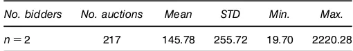
Table 1. Summary Statistics on Bids per Acre
No. bidders No. auctions Mean STD Min. Max.
nD2 217 145.78 255.72 19.70 2220.28
the corresponding bids in 1972 dollars. As an illustration, we consider auctions with two bidders only. We could consider auctions with a higher number of bidders, but the number of
corresponding auctionsLn tends to reduce dramatically. The
summary statistics of bids per acre are given in Table 1 for two bidders.
Table 1 indicates that there is a great variability in bids as measured by the standard deviation and the range of bids; a large proportion of bids falls between $50 and $200 per acre. A test for independence among bids within auctions using the Blum, Kiefer, and Rosenblatt (1961) nonparametric test gives a test statistic equal to 6.00 corresponding to ap-value equal to .14%. This constitutes a clear rejection of independence and hence of the IPV model. This leads us to consider the APV model.
As a rst approximation, we assume that the current reserve price is nonbinding and hence does not act as an effective screening device to participating to the auction because the reserve price of $15 per acre is much lower than the average bid. Moreover, very few bids are clustered around the actual reserve price of $15. Specically, less than .25% of bids are in the interval6151207 and less than 1% are in the interval
6151307. Hence, the actual reserve price can be viewed as non-binding. Second, the federal government sometimes rejected the highest bid in some auctions although that bid was larger than the announced reserve price. Hence, the actual reserve price can be viewed as random. For wildcat auctions between 1954 and 1969, we observe a 1.8% rejection rate for the 217 auctions analyzed here. We can reasonably consider that the random reserve price does not have much effect on bidding strategies.
Third, we assume that there is no dynamic consideration in these auctions. This can be justied by the fact that the different sales were spread widely over the 1954–1969 period, reducing dynamic linkages across sales. Within each sale, we follow the earlier literature, which neglects oil companies’ capacity constraints given their large sizes; see Porter (1995). Fourth, we have to address the possible heterogeneity across tracts because this affects the value of the optimal reserve price. To assess possible heterogeneity across tracts, we fol-lowed Porter (1995) and regress the log of bids on a com-plete set of tract-specic dummies. Using the full dataset of 1,147 auctions, we obtain a weak rejection of tract homogene-ity based on anF-test. Because the F-test requires indepen-dence among bids, this statistic tends to overreject the null assumption of homogeneity because bids are not independent in the presence of afliation. Moreover, a similar regression
controlling for the number of bidders shows that theF-value
drops signicantly. To assess further tract heterogeneity given a number of bidders, we conduct separate regressions for each size of bidders. We nd that tract dummies explain an even lower percentage of the variability of the log of bids. Hence, we can reasonably neglect heterogeneity among tracts when
controlling for the number of bidders. This is automatically satised because our econometric analysis is conducted sepa-rately for each number of bidders.
3.2 Practical Issues
We assume that the underlying joint density f 4v11 v25 is
twice continuously differentiable, that is, RD2. To
imple-ment our kernel estimators (8) and (9), we need to choose a kernel function. The triweight kernel has a compact
sup-port and two continuous derivatives. It is dened as K4u5D
435=32541ƒu253 4—u—µ15 and is of order 2 in agreement
with Assumption A2. FornD2, Equation (10) gives the
band-widths hGDcGLƒ1=5 andhgDcgLƒ1=6, where cG andcg are
some constants. These two constants are obtained by the so-called rule of thumb. Specically,cGDcgD209781006‘Ob,
where‘Ob is the empirical standard deviation of bids, and the
factor 2.978 is the correction for the triweight kernel; see Hardle (1991).
For inference purposes, it is useful to provide condence intervals for pOü0D O4xO05, where xO0 maximizes the estimated
expected prot (11). Because asymptotic distributions of esti-mators in structural models are frequently difcult to establish, bootstrap methods are commonly used as an alternative for constructing approximate condence intervals. See Horowitz (in press) for a survey on bootstrap methods. Our bootstrap procedure is as follows. We resample the original data for auctions with two bidders to obtain 500 datasets, each of size equal to 434 bids. For each resampled dataset, we apply our semiparametric estimator and thus obtain 500 different values for pOü
0. To construct a 90% condence interval, we use the
Efron (1979) method relying on percentiles. This method does not impose any symmetry restriction.
3.3 Empirical Results
Any determination of the optimal reserve price requires the
knowledge of the value of the auctioned object v0 for the
seller. On the other hand, this valuation must be nonnegative. Moreover, because the seller may receive negative prots if the reserve price is set below the seller’s valuev0, the seller is
always better off setting a reserve price abovev0. Hence we can infer that the federal government valuation is between $0 and $15 per acre. In the following, we provide an estimate of the optimal reserve price for both values $0 and $15 as well as for bootstrap condence intervals. The results are given in Table 2.
The bootstrap condence intervals are relatively tight. It is interesting to compare our results with the approximation found by McAfee and Vincent (1992) when considering a pure common value model with endogenous entry and stochas-tic parstochas-ticipation of bidders. McAfee and Vincent found that
Table 2. Optimal Reserve Price
Seller’s valuation pü
0 Con’dence interval
v0D0 $272.83 [$2180711$322033]
v0D15 $290.07 [$2240801$336046]
the reserve price should be approximately $600 in 1992 dol-lars, that is, about 40-fold the current level. To be compara-ble, the results in Table 2, which are in 1972 dollars, need to be divided by .339. For two bidders we nd that the opti-mal reserve price should be $805 with a condence interval
6$6451$9517whenv0D0. This discrepancy can be explained by the absence of correction for the winner’s curse in a private value framework: when considering a pure common value model, bidders have to adjust their bids downward rela-tive to their private estimates because of the winner’s curse. This can explain why we obtain somewhat greater optimal reserve prices. Both approaches agree, however, that the actual reserve price used by the federal government is far from being optimal.
The choice of the reserve price is an important instru-ment with which the federal governinstru-ment can take advantage of its monopoly power in the auction as a unique seller. A higher reserve price induces rms to bid more aggressively but increases the probability of the auctioned tract not being sold. The optimal reserve price balances these two opposite effects and maximizes the seller’s expected gain. Thus, in terms of economic policy conclusions, simulating the rst-price sealed-bid auctions with the optimal reserve rst-price is of great interest for assessing the potential gain for the federal government. Using the estimator proposed by Li et al. (2002), we can recover the bidders’ private values by using the
equal-ity vD4b5 given in (6) for 174 auctions as well as the
underlying distribution of private values. Because nonparamet-ric methods are used, some auctions had to be trimmed out because of boundary effects.
For the 174 auctions for which we are able to recover bidders’ private values, we simulate the oil companies’ bids following (3) when facing our estimated optimal reserve prices. As expected, rms bid more aggressively whenever their private values are above the reserve price, but some tracts remain unsold because of the higher reserve price. Table 3 gives the percentage of informational rents, notedIR, left to the winning oil companies for sold tracts. The informational rent in percentage is computed as the ratio of the winning bidder’s private value minus the bid divided by the bidder’s private value. We perform the simulation 500 times using resampled data to obtain condence intervals.
We observe that about half of the tracts remain unsold. Moreover, the informational rents decrease signicantly from the average informational rent under the actual reserve price, which is 62%. The latter gure is computed from the observed winning bids and the estimated private values for the 174 auc-tions. Hence, implementing the optimal reserve price would allow the federal government to be much more successful in capturing the willingness to pay of the oil companies.
Another issue of great interest is to compare revenues and prots between the two mechanisms. Table 4 gives the
Table 3. Average Informational Rents for the Optimal Reserve Price
v0 No. sold tracts Con’dence interval IR Con’dence interval
0 90 [851107] 43.87% [35033%145031%]
15 88 [771103] 39.31% [37024%145082%]
Table 4. Revenues in Dollars for an Average Sold Tract
Actual Optimal Con’dence
v0 mechanism mechanism interval
0 $5141184092 $112671528001 [$1108514980101$115681295060] 15 $5141184092 $114411549060 [$1110913380701$116011344060]
revenues from an average sold tract (in terms of acreage) and Table 5 gives the prots from an average sold tract for each mechanism. Again, we provide revenues and prots with the optimal reserve price when the federal government has a pri-vate value per acre equal to $0 or $15. Revenues are computed as the average winning bid times the average acreage of a tract, whereas prots are computed as the average winning bid minus the value of the tract for the federal government times the average acreage of a tract. We also provide 90% bootstrap condence intervals.
It is important to note that revenues and prots for an ave-rage sold tract both signicantly increase as expected. On the other hand, as noted, half of the tracts become unsold under the optimal reserve price. Nevertheless, if we multiply the gures in Tables 4 and 5 by the number of sold tracts, the overall prot and revenue for the federal government is much higher than those from the actual mechanism. For instance, if we assume that the value of a tract for the federal government is $15 per acre, the optimal reserve price would allow prots of around 50% larger than actual prots although more tracts remain unsold.
4. CONCLUSION
A well-known difculty in implementing optimal reserve prices on eld data is that the latent distributions are unknown to the analyst. In this article we circumvent such a difculty by showing that the seller’s expected prot can be expressed as a functional of the observed bids distribution. Hence, the seller’s expected prot function can be identied and esti-mated from observed bids. It follows that a natural estimator of the optimal reserve price can be obtained by maximizing the estimated prot function. This leads us to propose a semi-parametric extremum estimator of the optimal reserve price, which is shown to be strongly consistent. In addition to being more direct and computationally simpler, this estimator can converge at a faster rate than can one relying on the estima-tion of the underlying distribuestima-tion of private values.
Possible future lines of research are as follows. First, our estimation procedure does not impose any parametric assump-tions on the distribution of private values and hence on the observed bid distribution. A possible extension of our method is to specify a parametric family for the distribution of observed bids. Second, as mentioned, an alternative semipara-metric procedure would be to use the rst-order conditions
Table 5. Pro’ts in Dollars for an Average Sold Tract
Actual Optimal Con’dence
v0 mechanism mechanism interval
0 $5141184092 $112671528001 [$1108514980101$115681295060] 15 $4441756021 $113721968080 [$1104017570901$115321763090]
characterizing the optimal reserve price to develop a semi-parametric GMM estimator. Third, because our result relies on the identication of the model from which bids are generated, it would be interesting to consider bids arising from a rst-price auction with a binding reserve rst-price. Guerre et al. (2000) solved such an issue within the IPV paradigm, and Hendricks, Pinkse, and Porter (2000) considered the CV model. Fourth, as is the case for many auction situations, such as procurement auctions, our illustration involves a public seller. Because of its public nature, it may be possible that the seller has objec-tives other than prot maximization. Although of great inte-rest, this issue requires more theoretical research.
ACKNOWLEDGMENTS
The authors are grateful to K. Hendricks and R. Porter for providing the data analyzed in this article as well as to M. Pesendorfer, the editor, and two referees for helpful and constructive comments. This article was presented at the Far Eastern Meeting of the Econometric Society in Singapore, June 1999, and at the Winter Meeting of the Econometric Society in Boston, January 2000. Financial support from the National Science Foundation under grant SES-0001663 to the rst author and grant SBR-9631212 to the third author is gratefully acknowledged.
APPENDIX
A.1 Proofs of Theoretical Results
Proof of Proposition 1. Using an argument similar to that by Riley and Samuelson (1981), we maximize the expected prot for the seller. For any bidder, say, Bidder 1, the expected payment if he or she wins the auction givenv1¶p0is
p4v15Ds4v11 p05Pr 4v2µv11 : : : 1 vnµv1—v15
Ds4v11 p05Fy1—v14v1—v151 (A.1)
where s4v11 p05 is given by (3). Therefore, using (3), the expected revenue for the seller from Bidder 1 is
R14p05DZv
p0
p4v15f 4v15 dv1
DZ
v
p0
µ
v1ƒZ
v1
p0
L4—v15 d
¶
Fy1—v14v1—v15fv14v15 dv10 (A.2)
The total expected prot ç for the seller is the sum of the
seller’s private value for the object if the latter remains unsold and the expected revenue for the sellers if it is sold to any of
then bidders. Because of the symmetry among bidders, we
obtain
ç4p05Dv0F 4p01 : : : 1 p05CnR14p050 (A.3)
Differentiatingç4p05with respect top0, the expected prot of
the seller is maximized for somepü
0 satisfying the rst-order
condition
nFy1—v14p
ü
0—p0ü5fv14p
ü
054v0ƒpü05 Cn
Zv
pü
0
L4p0ü—v15Fy1—v14v1—v15fv14v15 dv1D01
because dF 4x1 : : : 1 x5=dxDnFy
1—v14x—x5fv14x5. Equation (4)
follows.
Proof of Proposition 2. Combining (3), (A.1), (A.2), and (A.3), and using y1Dmaxj6D1vj, the expected prot for the
sellerç4p05is equal to
ç4p05Dv0E6 4y1µp05 4v1µp057
CnZ v
v
4v1¶p05s4v11 p05
³Zv
v
4y1µv15fy1—v14y1—v15 dy1
´
fv14v15 dv1
DE6v0 4y1µp05 4v1µp05
Cns4v11 p05 4y1µv15 4v1¶p0570 (A.4)
Now, forp0andv1such thatvµp0µv1µv, we have from (2) and (3)
s4v11 p05Ds4v15CZ
p0
v
L4—v15 d
Ds4v15CL4p0—v15Z p0
v
L4—p05 d
Ds4v15CL4p0—v154p0ƒs4p0551 (A.5)
where the second equality follows from L4—v15DL4—p05 L4p0—v15 and the third equality follows from (2) evaluated at
viDp0.
Because p0 D 4x5 and v1 D4b15, L4p0—v15 is also
equal to L44x5—4b155. The latter is denoted å4x—b15 and can be expressed as a function of the observed bids distribution. Specically, let Fy1v14y1 v5DFy1—v14y—v5fv14v5.
Because Fy1v14t1 t5 D GB1b14s4t51 s4t55 and fy11v14t1 t5 D gB11b14s4t51 s4t55s
04t5, using a change of variableuDs4t5, we obtain
å4x—b15²L44x5—4b155 Dexp
³ ƒZb1
x
gB11b14u1 u5 GB1b14u1 u5
du
´
0 (A.6)
Combining (A.4), (A.5), and (A.6), and usingB1Ds4y15,b1D
s4v15,p0D4x5,xDs4p05withs4¢5increasing, (A.4) can be
written as in (7), as desired.
A.2 Proofs of Statistical Results
We make the following assumptions. Throughout we assume thatn¶2.
Assumption A1. For each n¶2, the private values vec-tors4V1`1 : : : 1 Vn`51 `D1121 : : : 1are independently and
iden-tically distributed (iid) with joint density f 4v11 : : : 1 vn5. The latter hasR¶1 continuous partial derivatives on6v1 v7n with f 4v11 : : : 1 vn5¶c >0 on 6v1 v7n.
Assumption A2.
1. The kernelK4¢5is symmetric with support6ƒ11C17with continuous bounded rst and second derivatives.
2. RK4u5duD1.
3. K4¢5is of orderRCnƒ2 (RC1 for the IPV case), that is, moments of order strictly smaller than the given order vanish.
Note that Assumption A1 implies that the bids vectors
4B1`1 : : : 1 Bn`51 ` D1121 : : : 1 are iid. Note also that the
marginal densityf 4¢5²fv14¢5hasRcontinuous derivatives on 6v1 v7and thatf 4¢5¶c >0 on6v1 v7. Moreover, Assumption
A1 implies thatv <ˆso thatb <ˆ.
The next lemma states the uniform consistency of the non-parametric estimators (8) and (9) ofGB1b14¢1¢5andgB11b14¢1¢5,
respectively, on arbitrary xed compact inner subsets of their supports as well as on expanding subsets. This lemma was
proved by Li et al. (2002, lem. A5). Let £ be an arbitrary
but xed inner compact subset of 6b1 b7, and let £
L be the
expanding subset6bC„1 bƒ„7, where„Dmax8hG1 hg9 with
4hG1 hg5dened by (10).
Lemma A.1. Under Assumptions A1 and A2 with R¶1, we have
1. sup£2—GbBbƒGBb— DO4hGRCnƒ25, sup£2—OgB1bƒgB1b— D O4hRCnƒ2
g 5,
2. sup£L2—GbBb ƒGBb— D O4hRG5, sup£L2—OgB1b ƒgB1b— D O4hR
g5.
As is well known, the convergence rate in part 2 of Lemma A.1 is slower than that in part 1 because of boundary effects in nonparametric estimation.
Next, we need another lemma similar to Theorem 4.1.1, of Amemiya (1985) which is fundamental for establishing the consistency of extremum estimators. In addition to allowing a discontinuous statistical objective function, our lemma allows for maximization and uniform consistency over an expanding subset.
Lemma A.2. Let Q4¢5 and QL4¢5 be nonstochastic and
stochastic functions dened on the compact setsä and äL,
where äL forms an increasing sequence of possibly
stochas-tic subsets of ä converging almost surely to äo so that
äo²[ˆ
LD1äL almost surely. For everyLD1121 : : :, letˆOLbe
a value inˆ satisfying
QL4ˆOL5¶sup ˆ2äL
QL4ˆ5O Co4150
If (i)Q4¢5is continuous onäwith a unique maximizer onä
atˆ02äo and (ii) sup
ˆ2äL—QL4ˆ5ƒQ4ˆ5— !0 almost surely
as ! ˆ, thenˆO!ˆ0 almost surely.
Proof of Lemma A.2. Adapting it to our case, the proof is largely inspired by the proof of Theorem 4.1.1 in Amemiya
(1985). LetN be an arbitrary (open) neighborhood ofˆ0 and
letNSbe its complement inä. Let
‡DQ4ˆ05ƒmax
ˆ2 SN\ä
Q4ˆ50 (A.7)
Thus‡ >0 because ˆ0 is the unique maximizer of Q4¢5 and
Q4¢5is continuous on the compactN\ä.
Now, from (ii) we have almost surely for allL sufciently
large supˆ2äL—QL4ˆ5ƒQ4ˆ5—< ‡=3. But, we have almost
surelyˆ02äLfor allLsufciently large asˆ02äoD [ˆ
LD1äL.
Hence, applying the preceding inequality at ˆDˆ0 and ˆD
O
ˆ2äL, we obtain almost surely for allL sufciently large
Q4ˆ5 > QO L4ˆ5O ƒ‡=31 (A.8) QL4ˆ05 > Q4ˆ05ƒ‡=30 (A.9)
On the other hand, we have supˆ2äLQL4ˆ5 ¶ QL4ˆ05
because, as noted,ˆ02äL for allLsufciently large. Hence, using the denition ofˆO we haveQL4ˆ5O ¶QL4ˆ05Co415. We
can pick Ln sufciently large so that o415 >ƒ‡=3. Hence,
almost surely and for allLsufciently large, we haveQL4ˆ5 >O QL4ˆ05ƒ‡=3. Using (A.9), it follows that QL4ˆ5 > Q4ˆO 05ƒ
2‡=3. Using (A.8), it follows thatQ4ˆ5 > Q4ˆO 05ƒ‡. Hence,
using (A.7), it follows thatˆO2N\äalmost surely. Indeed, for allˆ2N\ä, we haveQ4ˆ5µmaxˆ2N\äQ4ˆ5DQ4ˆ05ƒ‡.
Proof of Proposition 3. It sufces to show that the
assump-tions of Lemma A.2 are satised with LDLn, äD6b1 b7,
äLD6bminC„1 bmaxƒ„7,Q4¢5Dç4¢5, andQL4¢5Dç4b ¢5. Note
that bmin#b, bmax "b and „#0 almost surely as Ln! ˆ.
Hence, äL forms an increasing sequence of compact subsets
ofäconverging toäoD4b1 b5almost surely.
Regarding (i), ç4¢5 is clearly continuous on ä in view of
(7) and Assumption A1. Moreover, becausepü
0n is the unique
maximizer of the seller’s expected prot on6v1 v7, and because
x0n Ds4p0ün5, then ç4¢5 admits a unique maximizer on äD
6b1 b7atˆ0Dx0n. Becausev < pü0n< vby assumption ands4¢5
is strictly increasing, thenb < x0n< b, that is,x0n2äo.
Regarding (ii), Assumption A1 and the abstract Glivenko– Cantelli theorem (van der Vaart 1998, p. 270) imply
1
Ln Ln
X
`D1
1
n n X
iD1
v0 4Bi`µx5 4bi`µx5
!v0GB11b14x1 x51 (A.10)
1
Ln Ln
X
`D1
1
n n X
iD1
nbi` 4Bi`µbi`5 4xµbi`5
!n Zb
x
tGB1b14t1 t5 dt (A.11)
uniformly in x2ä almost surely as Ln ! ˆ. Following
Example 19.6 of van der Vaart (1998), it can be readily shown that the bracketing numbers of families of functions of the form v0 4Bµx5 4b µx5 or b 4B µb5 4xµb5, where
x2ä, are nite. Turning to the third term in (11), we rst
recall from the proof of Proposition A2 of Li et al. (2002) that
sup
x26bC„1bƒ„7
b
GB1b14x1 x5
O
gB11b14x1 x5
ƒGB1b14x1 x5 gB11b14x1 x5
µO4hRƒ4nƒ25
g 50 (A.12)
BecauseäL 6bC„1 bƒ„7 almost surely asL! ˆ, it
fol-Moreover, from Li et al. (2002, lem. A2) we also have
GB1b14x1 x5
gB11b14x1 x5 Da4xƒb5Co4xƒb51 (A.13)
where aD1=4nƒ15 so thatGB1b14x1 x5=gB11b14x1 x5 is
con-tinuous inx26b1 b7.
Thus, dropping the subscript i because of symmetry, it
remains to study the almost sure uniform convergence on
6bminC„1 bmaxƒ„7of
We now study the three terms on the right-hand side, denoted
A14x5,A24x5, and A34x5.
where we dropped the argument 4u1 u5 to simplify. From
(A.13) and Lemma A6 of Li et al. (2002) we have infu26bC„1bƒ„7GB1b14u1 u5=gB11b14u1 u5 ¶ c„, where c > 0.
Thus, if R¶n as assumed, it follows from (A.12) that the
rst term is uniformly strictly positive and dominated by 1=6c„CO4„Rƒ4nƒ2557 for sufciently large L
n, almost surely.
Because the second term is anO4„Rƒ4nƒ255 by (A.12), it
fol-lows thatã4u5DO4„RƒnC15uniformly in u26bC„1 bƒ„7.
Hence, for… arbitrarily small, we have—ã4u5—µ…uniformly in u26bC„1 bƒ„7 for Ln sufciently large, almost surely. Thus
å4r—t51C…ƒå4r—t5µbå4r—t5ƒå4r—t5µå4r—t51ƒ…ƒå4r—t5
uniformly in 4r 1 t5 such that bC„µr µtµbƒ„ for Ln
sufciently large, almost surely. But the functions x1C…ƒx
and x1ƒ…ƒx attains their minimum and maximum on 60117
Because the lower bound and upper bound converge to zero
as …!0, and because … can be chosen arbitrarily small, it
follows that supbC„µrµtµbƒ„—bå4r—t5ƒå4r—t5— !0 asLn! ˆ,
almost surely. Hence supx26bC„1bƒ„7—A14x5—µ0 as Ln! ˆ,
almost surely.
Next, considerA24x5. From the abstract Glivenko–Cantelli
theorem (van der Vaart 1998, p. 270) we obtain A24x5!
E6å4x—b5 4Bµb5 4xµbµb57uniformly inx2äD6b1 b7,
asLn! ˆ, almost surely. Combining Examples 19.6 and 19.7
of van der Vaart (1998), it can be shown that the bracketing
numbers of families of functions of the form å4x—b5 4Bµ
b5 4xµbµb5, where x2ä, are nite. Note that the right-hand side is continuous onä.
Last, considerA34x5. Because 0µå4r—t5µ1, we have from the standard Glivenko–Cantelli theorem that the
right-hand side converges almost surely to zero asLn! ˆ. Hence
supx2ä—A34x5— !0 asLn! ˆ, almost surely.
Collecting results, it follows from (A.12) and (A.14) that
b ing (A.10), (A.11), and (A.15) into (11) and using (7) show thatç4x5b !ç4x5, uniformly inx2äLD6bminC„1 bmaxƒ„7, asLn! ˆ, almost surely. This establishes (ii) of Lemma A.2 and hence Proposition 3.
A.3 The IPV Case
A Reformulation from Observed Bids. Proposition 2 applies a fortiori to the IPV case. In this case, the inverse bid-ding strategy4¢5in (6) reduces to
4b5DbC 1
nƒ1
G4b5
g4b51 (A.16)