CAPITAL INTENSITY, OPENNESS, AND THE ECONOMIC GROWTH OF
THE ASEAN 5
Ni Putu Wiwin Setyari
Faculty of Economics and Business, Universitas Udayana, Indonesia ([email protected])
Surya Dewi Rustariyuni
Faculty of Economics and Business, Universitas Udayana, Indonesia ([email protected])
Luh Putu Aswitari
Faculty of Economics and Business, Universitas Udayana, Indonesia ([email protected])
ABSTRACT
One of the core elements of the neoclassical growth theory is that poor countries have low capital-labor ratios but have higher marginal products of capital than the rich countries. This means the low-income countries experience faster growth rates and become a reason for allowing capital, goods, and technology can move across countries. Assuming that the labor intensive countries have higher returns on capital, then investment will flows into those countries and encourage higher economic growth. However, in fact capital flows seems to go in the opposite direction. A country with abundant capital can expand its capital-intensive sectors and export their goods along with trade liberalization. Consequently, the returns to capital in its capital-intensive sectors rise and a greater demand for investment induces higher capital inflows from abroad. Those predictions push developing countries to change their labor intensive industrial structures and become more capital intensive, to encourage their economic growth. This paper examines how capital intensity and openness affect economic growth using data from the ASEAN 5 countries data. The issue of endogeneity and unobserved heterogeneity, as major problems in a data panel, are addressed by the fixed effect method and the Feasible General Least Square (FGLS). Capital flows appears to be the most important source of economic growth, whilst trade is found to have a limited role. The interaction between capital intensity and the openness indicator do not indicate significant effects. Generally, there is no evidence that the more outward-oriented countries with high levels of capital intensity experiences higher economic growth.
Keywords: foreign direct investment, economic growth of open economies, capital intensity of industrial structure, and impact of globalization
JEL Classification: F21, F43, E22 F62
INTRODUCTION
The idea that economic openness is the most important determinant of economic growth is becoming increasingly popular among develop-ing countries. Open, in Foreign Direct Investment (FDI) and trade, is often seen as an important catalyst for economic growth in the developing countries (Makki & Somwaru, 2004). Many studies suggest that a more
countries from 1980 to 1990. That study’s result suggested a significantly positive relationship between openness and productivity’s growth. Therefore, market-oriented economic policies, including the liberalization of international trade and capital flows, became the center of the economic reform efforts, including in Asia. According to Wacziarg and Welch (2003) the percentage of countries open to trade increased from 16 to 73 percent between 1960 and 2000. Braun and Raddatz (2007) also show from the 108 countries in their sample, the number of countries that allow free trade grew from 24 to 88 in the case of goods, and from 10 to 47 for capital.
Most of the developing countries adopt capital liberalization to stimulate economic growth by attracting foreign investment. It is consistent with economic thought that capital would be more beneficial when it (capital) can moves freely across countries to find the most productive investments (Bailliu, 2000). The result of a study by Henry (2003) shows that the liberalization of the capital accounts has a positive effect on growth because it reduces the cost of capital. However, the study by Caporale and Giraldi (2012) shows trade connection appears to be the most important source of the business cycle’s co-movement, whilst capital flows are found to have a limited role, especially in the very short-term.
The evolution of the growth theory tries to identify the relationship between economic openness and the growth rate, one facet of which is the endogenous growth model that explains the existence of a direct link between openness and growth rates, which are not described in the neoclassical growth model (Gundlach, 1997). Edwards (1993, 1997) uses this model and finds a positive relationship between openness and the economic growth rate (measured by the Total Factor Productivity/TFP) as a result of the adop-tion of technological innovaadop-tions. However, this theory is unable to explain the empirical evidence for the conditional convergence’s existence.
Conditional convergence is defined as a condition in which a poor economy tends to
grow faster than a richer economy when various determinants assume a constant steady state (Barro & Sala-i-Martin, 2004). Conditional convergence is predicted by the neoclassical theory. However, the main weakness is the assumption of a closed economy. It then develops into an open economy that allows capital flows (Gundlach, 1997). This model predicts that when adjusted to a steady state, an open economy grows to be larger than a closed economy because it can acquires capital more quickly from the international financial markets.
The other core element of the neoclassical growth theory is poor countries, which have a low capital-labor ratio, have higher marginal products of capital than the rich countries. Its means the low-income countries experience faster growth rates and become a reason for allowing capital and technology move across countries (Barro, 1991). This raises the question of whether the capital-poor countries which are open to the global economy grows faster than the open rich countries. Heckscher-Ohlin pre-dicts if a country has a total labor force greater than its capital, it will have a comparative advantage in labor-intensive products and thus the industrial structure tends to be labor-intensive. Assuming that a labor-intensive coun-try has a higher return on capital, then invest-ment will flow into this county and encourage higher economic growth. In other word capital will flow from developed countries to developing countries. In fact, foreign direct investment seems to take the opposite direction (Jin, 2012). He explicitly expresses that foreign capital will flow into a country with capital-intensive industries. With its trade in goods, a capital abundant country can expand its capital-intensive sectors and export their goods in response to any labor force/productivity boom in other countries. Consequently, the returns to capital in its capital-intensive sectors rise and a greater investment demand induces higher capital inflows from abroad.
countries with highly labor intensive production systems, and greater openness generate lower inequalities in response to favorable shocks. Using data from 42 low to middle income countries, the result shows that the key to understanding whether trade openness and foreign investment have negative or positive effects on inequality depends on the dynamics between wages and profits, and the degree of labor intensity in the production cycle. However as we known, there is no previous study which focuses on openness and capital intensity’s interaction effects on growth, especially for the ASEAN 5.
Economic growth in the region of the Association of Southeast Asian Nations (ASEAN) has become part of the East Asian miracle (Park et al, 2008). Singapore became a new industrial economy along with Hong Kong, Korea, and Taiwan. The East Asian miracle consists of the fact that a group of small export-oriented economies have been able to grow at rates that are so high (Ventura, 1997). Mean-while Indonesia, Malaysia and Thailand have been transformed from agricultural countries into dynamic manufacturing countries through sustainable growth and industrialization. Other ASEAN economies have also begun to achieve relatively fast and consistent growth.
ASEAN was founded in 1967 by Indonesia, Malaysia, the Philippines, Thailand, and Singapore, which are known as the ASEAN-5. Brunei joined in the 1980s, to form the ASEAN-6, which was joined by Cambodia, Laos, Myanmar and Vietnam (known as CLMV) in the 1990s. All ASEAN members have differences in their size, the rate of their economic growth, their resources, and in the capabilities of their technology and industries (Yue, 2004). In 1992, ASEAN agreed to establish the ASEAN Free Trade Area (AFTA) with a tariff reduction to 0% - 5% in 2002 for the ASEAN-6. The tariff was reduced to zero in 2010 for the ASEAN-6 and for the CLMV in 2015. In addition, ASEAN also has a liberalization agreement for its services and investments, and agreement for free trade with China, Japan, South Korea and India, while each of its members form bilateral free trade
deals with a number of countries in the Asia Pacific region and beyond (Shiino, 2012). This shows the high level of the ASEAN countries’ openness.
The analysis in this paper emphasizes the openness and capital intensity’s effect on economic growth in the ASEAN 5. To analyse the data, the paper adopts the Autoregressive Distributed Lag model (ARDL) developed by Pesaran et al. (2001). The main advantage of this method is that it yields valid results irrespective of whether the underlying variables are I(0), I(1), or a combination of both (Pesaran & Shin, 1997). A fixed effect model is combined with a three steps feasible least square used to overcome endogeneity issues, even though the Granger test shows no causality effects from the explanatory variables to GDP’s growth as a dependent variable. The result indicates if the openness, especially in foreign direct invest-ment, and capital intensity, affect the economic growth. However, the interaction between capital intensity and openness suggests there is no evidence the more outward-oriented econo-mies with more capital intensity experience higher economic growth.
LITERATURE REVIEW
number of economies in East Asia have actually succeeded in raising their levels of per capita income to those of the DCs (Lin & Zhang, 2009).
Lin (2003) argues that the failure of most LDCs to converge with the DCs in terms of their economic performance can be largely explained by their governments’ inappropriate develop-ment strategies. Most LDC governdevelop-ments pursue development plans that place a priority on the development of certain capital-intensive indus-tries. However, an economy’s optimal industrial structure is endogenously determined by that economy’s endowment structure. Often the firms in a government’s priority industries are not viable in an open, competitive market because these industries do not match the comparative advantage of their particular economy. As such, the government introduces a series of distortions in its international trade, financial sector, labor market, and so on, to support these non viable firms. It is possible with such distortions to establish capital-intensive industries in develop-ing countries, but the economy becomes very inefficient because of the misallocation of resources, rampant rent seeking, macro instabil-ity, and so forth. Consequently, convergence - that is, the convergence of the LDC’s economic indicators to levels akin to those of the DCs - fails to occur. By contrast, the LDC’s govern-ments, e.g. the newly industrialized economies in Asia and more recently China, may pursue a comparative-advantage-following strategy. In this strategy, a government attempts to induce a firm’s entry into a industry according to the economy’s existing comparative advantage, and to facilitate the firm’s adoption of appropriate technology by borrowing at low cost from the more advanced countries (Lin & Zhang, 2009).
The hypothesis that poor countries tend to grow faster than rich countries seems to be inconsistent with the cross-country evidence found by Barro (1991) using data from 98 countries over the period 1960-1985, which indicates that per capita growth rates have little correlation with the starting level of per capita products. Moreover, given the level of initial per capita GDP, the growth rate is substantially
positively related to the starting amount of human capital. Thus, poor countries tend to catch up with rich countries if the poor countries have high human capital per person (in relation to their level of per capita GDP), but not otherwise. As a related matter, countries with high human capital have low fertility rates and high ratios of physical investment to GDP. Barro (1991) also found per capita growth was negatively related to the ratio of a government’s consumption expenditure to the country’s GDP. An interpretation is that government consump-tion introduces distorconsump-tions, such as high tax rates, but does not provide an offsetting stimulus to growth.
Since 1960 Asia, the largest and most populous of the continents, has become richer faster than any other region of the world. Of course, this growth has not occurred at the same pace all over the continent. The western part of Asia grew during this period at about the same rate as the rest of the world, but, as a whole, the eastern half (ten countries: China, Hong Kong, Indonesia, Japan, Korea, Malaysia, the Philippines, Singapore, Taiwan, and Thailand) turned in a superior performance. The worst performer was the Philippines, which grew at about 2 percent a year (in per capita terms), about equal to the average of the non-Asian countries. China, Indonesia, Japan, Malaysia, and Thailand did better, achieving growth rates of 3-5 percent (Sarel, 1996).
Nelson and Pack (1999) distinguish between two groups to explain the Asian miracle. Firstly is the "accumulation" theory that emphasizes the role of physical investment in moving these economies along their production function. Secondly, the "assimilation" theory, which focuses on an economy’s entrepreneurship, innovation and learning of new technology which is adopted from the advanced industrial nations. They predict as capital and labor shift to the modern sector, that capital intensity will increase (Nelson & Pack, 1999).
equili-brium model they show that differences in the factor proportions across sectors combined with capital deepening leads to non balanced growth, because an increase in the capital-labor ratio raises output more in the sectors with the greater capital intensity, whereas the output value and employment grow more in the less capital-intensive sectors. Moreover, they show that capital and labor are continuously reallocated away from the more rapidly growing sector. Cipollina et al. (2011) highlights three major explanations of why FDI may potentially enhance the growth rate at the industry level in the host country: Technological innovation, labor accumulation, and capital accumulation. Their analysis provides evidence of positive and statistically significant effects of FDI on the rate of growth of the industries in host countries, and shows that this effect is stronger in capital intensive sectors, and in sectors with higher levels of technological development. A similar result is also suggested by Jin (2012), who states that foreign capital flows into countries with capital intensive industries.
The East Asian economies have substantially liberalized their foreign trade and direct investment (FDI) regimes within the framework of the General Agreement on Tariffs and Trade (GATT)/World Trade Organization (WTO) and the Asia-Pacific Economic Cooperation (APEC). It traces East Asia’s rise to the coveted “Factory Asia” league with rapid growth over several decades through trade policies anchored on outward-oriented industrialization strategies (Kawai & Wignaraja, 2014). It is well known that free trade, or the liberalization of trade via a reduction of the impediments to imports (tariffs, NTBs) and exports, are the best strategies from a welfare point of view. These welfare improve-ments are due to specialization gains (increased efficiency due to production according to comparative advantage) and to consumption gains (increased choice of goods at lower prices for consumers) (Nowak, 2000).
The modern theory of trade policy, in terms of trade restrictions’ relationship to GDP, can be summarized in the following three propositions (Rodriguez & Rodrik, 2001): 1) In static models
with no market imperfections and other pre-existing distortions, the effect of a trade restriction is to reduce the level of real GDP at world prices. In the presence of market failures such as externalities, trade restrictions may increase real GDP; 2). In standard models with exogenous technological changes and diminish-ing returns to reproducible factors of production (e.g., the neoclassical model of growth), a trade restriction has no effect on the long run (steady-state) rate of growth of output. This is true regardless of the existence of market imperfec-tions. However, there may be growth effects during the transition to the steady state. These transitional effects may be positive or negative, depending on how the long-run level of output is affected by the trade restriction.3). In models of endogenous growth generated by non-diminishing returns to reproducible factors of production or by learning-by-doing and other forms of endogenous technological changes, the presumption is that lower trade restrictions boost output growth in the world economy as a whole. However, a sub-set of countries may experience diminished growth, depending on their initial factor endowments and levels of technological development.
output is neither a necessary nor a sufficient condition for an improvement in welfare.
Grossman and Helpman emphasized the ability of trade to promote innovation in a small open economy depends on whether the forces of comparative advantage push the economy's resources in the direction of activities that generate long run growth (via externalities in research and development, expanding product varieties, improving product qualities, and so on) or diverts them from such activities (Rodriguez & Rodrik, 2001).
Baldwin and Seghezza (1996), who at-tempted to indentify the mechanisms linking trade and growth, particularly used a theoretical model that establishes a link between trade liberalization and investment-led growth. The theoretical model assumes each country has a traded and non-traded goods sector with the traded goods sector being relatively capital intensive. The model also assumes that traded goods are an intermediate input into the production of new capital. In this model domestic protection creates conflicting influ-ences on the steady-state capital-labor ratio. Estimating equations are derived from the model and estimated with three stage least squares on a cross-country data. Analysis of the result found that domestic protection depresses investment and thereby slows growth. Foreign trade barriers also lower domestic investment, but the anti-investment effect is weaker and is less robust to sample and specification changes.
Daumal and Özyurt (2011) explored the impact of trade openness on the economic growth of Brazilian states according to their initial income levels over the period from 1989 to 2002. The results indicated that openness is more beneficial to states with a high level of initial per capita income and therefore contri-butes to increased regional disparities. In addition, trade openness favors more industria-lized states, well-endowed in human capital, rather than states whose economic activity is mainly based on agriculture.
DATA AND METHODOLOGY
The data used in this research are panel data from the ASEAN 5 countries namely Indonesia, Malaysia, the Philippines, Singapore, and Thailand. Major focuses here are on their indus-trial structures and the effects of their openness on their economic growths. The dynamic trade theory is based on neoclassical assumptions and is mainly verbal in character. Dynamic gains are caused by an accelerated accumulation of physical capital and human capital (perhaps due to a higher rate of domestic and/or foreign savings), enhanced technological transmissions and improvements in the quality of macroeco-nomic policies. In contrast to the static traditional trade theory which emphasizes the efficiency gains from trade, the dynamic trade theory draws attention to the indirect gains from trade. The above-mentioned dynamic gains manifest themselves in increased growth rates of output in the medium and long-run (Nowak, 2000).
The dynamic panel data model is characte-rized by the lagged dependent variable’s presence as one of the independent variables. The model is as follows:
= + , + + +
+ + (1)
Economic growth is represented by yit which is a
country’s annual growth in its GDP from 1980 until 2014. Variable CIit is the capital intensity’s
growth of country i at period t. Capital intensity is constructed as a ratio of the capital stock - labor force. A higher capital intensity value indicates the capital endowment increases higher than the labor force. A country with a high capital intensity value will tend to specialize in capital intensive industries, in which they have a comparative advantage. The inclusion of the lagged values of the dependent variable as a regressor is a means of simplifying the form of the dynamic model (which would otherwise tend to have a large number of highly correlated lagged numbers of correlated lagged values of X); by replacing restrictions on how current Yt
adjusts to the lagged values of Xt-j (j = 0, ….,q) it
entering the estimated equation, at the cost of some extra lagged terms involving Yt-j (Harris,
1995). This is described in Koyck’s transforma-tion (Gujarati & Porter, 2009). The value of λ,
such that 0 < λ <1, is known as the rate of decline, or decay, of the distributed lag and where 1 – λis known as the speed of adjustment.
There are two ways to obtain a series of capital stocks (Shirotori et al., 2010): 1) Direct measurement by survey, and 2) the Perpetual Inventory Method (PIM). This research used the PIM method to estimate the capital stock in each country with the following formula:
t the depreciation rate. Problems that often arise are in the initial capital stock’s estimation and the depreciation rate’s assumption. In this research, the initial capital stock (K0) is
estimated by a disequilibrium approach. This approach uses the neo-classical growth theory and is based on the assumption that an economy is often at an adjustment position in its equili-brium path. Because of the adjustment process, the investment and capital accumulation tend to follow a systematic pattern. This assumption is considered more plausible than the assumption that the economy is in a steady state (Berlemann & Wesselhöft, 2012). The initial capital stock can be calculated with the following formula (Hall & Jones, 1999):
GFK
The gross fixed capital formation’s growth rate is calculated from the average growth rate of the gross fixed capital in the first ten years. The depreciation rate is generally assumed to be constant and equal across countries. However this is deemed inappropriate due to the fact that the richer countries will have a higher capital depreciation rate. The analysis in this study uses the depreciation rate listed in the Penn World Tables (PWT) 8.0 which varies across countries and time periods (Inklaar & Timmer, 2013).
Tradeit is the ratio of the international trade
(total exports plus imports) to GDP of country i
at period t, and reflects the country's trade openness. FDIit is the international capital flows
that specifically reflects the net foreign direct investment inflows value recorded in the balance of payments to GDP (in millions of USD) of country i at period t. is a set of other explana-tory variables as indicated by Barro (1991) as determinants of economic growth, namely the growth in government expenditure, which reflects the fiscal policy, the level of life expec-tancy which reflects the level of human capital, and the ratio of M2 to GDP which is an indicator of the development of the financial institutions which could also reflect the country’s monetary policy. Also regarded as an important determi-nant is the ratio of the productive population, that is the people aged 15 – 64 years old. This group is the active, productive population who work for a wage or salary, and at the same time act as savers to increase the capital accumula-tion.
depends on the development or acquisition of practical skills to get the job done more quickly and more efficiently (Sarel, 1996).
There are many potential channels through which openness may affect the GDP, but the direction of causation is also not clear. A great deal of literature documents Foreign Direct Investment (FDI) and trade as important determinants for economic growth in the developing countries especially (for example, the review in Lim, 2001; Makki & Somwaru, 2004). FDI has effects through many channels, such as it being a means for technology’s transfer from developed countries to developing countries. FDI also stimulates domestic investment and facilitates improvements in the human capital and the institutions of the host countries. International trade is also known to be an instrument of economic growth. Trade facilitates the more efficient production of goods and services by shifting production to countries that have a comparative advantage in producing them. While other studies, such as Rodrik (1999) and Jin (2012), have suggested that FDI tends to be located in more productive and faster-growing economies. On the other hand, the volume of trade is affected by trade policies. To the extent that trade restrictions represent policy responses to real or perceived market imperfec-tions or, at the other extreme, are mechanisms for rent extraction, they will work differently from the natural or geographical barriers to trade and other exogenous determinants (Rodriguez & Rodrik, 2001).
A common technique to solve the problem is to include individual effects in the model using a Fixed Effects Estimation Method (FEM). In the FEM, unobservable individual effects are assumed to be unchanged over time, while is assumed to be independent and identically distributed. However, the FEM has a weakness due to the loss of degrees of freedom (df) because of the inclusion of a dummy parameter, therefore we can only capture country-specific effects through a cross-section specific and try to save the degrees of freedom by modeling the common slope parameters. Additionally, the FEM cannot estimate the effects of variables that
are not changed over time, although it is relevant in the analysis of, such items as gender, race, religion, school, or geographic location.
Another problem to deal with is the homoscedastic nature of , which is not correlated over time. There are a number of statistical techniques that can address this problem, one of which is the weighted least squares method (Medvedev, 2006).
The consequences of autocorrelation are similar to heteroscedasticity, but the problems caused by the latter are usually more severe. The OLS coefficient estimates remain consistent and unbiased in the presence of autocorrelation, but they are no longer the Best Linear Unbiased Estimators (BLUE) or asymptotically efficient. In case both heteroscedasticity and autocorrela-tion are present in the data, a three-step FGLS approach is required, further complicating comparisons with the OLS/LSDV-type models. We employ estimation methods that remain consistent in the presence of panel-level heteroscedasticity and autocorrelation.
RESULT AND DISCUSSION
Before doing further analysis, we must know the nature of the data or variables used by the unit root test. A unit root test is intended to determine whether the data used are stationary or not, to avoid spurious regressions. If the variables used have unit roots and are not stationary, except when the data is combined with other non-stationary data to get a stationary cointegration, then regressions involving these data imply a mistake has occurred, in terms of the economic relationships (Harris, 1995). However, one advantage in panel data’s use is it is able to avoid a spurious regression (Baltagi, 2005). Unlike the spurious regression from the time series data, spurious regression estimations from panel data still give consistently correct estimations of value. This is due to the average estimator of the individual panels and information in cross-section data directs to the overall signal stronger than the time serial data.
Pesaran, and Shin (IPS) tests to test for the individual unit root’s presence for each item of the cross sectional data. Meanwhile for the panel data we use Levin, Lin, and Chu (LLC). The unit root test results are summarized in Table A.1 (Appendix).
The unit root test results show that the variables used in this study are stationary at different degrees. GDP’s growth, capital’s intensity, trade, and government expenditure are stationary at level or integrated into the I(0),
while others are stationary at the first difference or integrated into the I(1). Due to the linear combination of variables involving different degrees of integration, then the data with the highest degree of integration will be integrated with a series of variables that have the lowest degree of integration (Pagan & Wickens, 1989). Regressions using data on level will provide invalid estimation results and cannot be interpreted (Insukindro & Sahadewo, 2010).
Time Series Evidence
First, we try to test the effect of openness and industrial structures on economic growth in the time series data for each ASEAN 5 country. The application of the time series and panel data together are not comparable, due to the differences in the nature of the data, but they are at least able to give a better picture if both are present. Time series data analysis uses a dynamic regression Error Correction Mechanism (ECM). It is intended to capture the dynamism of short-term movements of the equilibrium path of economic growth, as well as from the panel data’s analysis. However, many advantages can be gained from the use of the ECM (Harris, 1995). First, the ECM incorporates both short-run and long-short-run effects that can provide information on the speed of adjustment, which is the dependent variable’s response to disequili-brium. Second, all the terms in the model are stationary, so the standard regression techniques are valid. Third, the ECM is closely bound up with the concept of co-integration. The ECM model in this analysis is as follows:
∆ = ∆ + ∆ + −
1 − − − −
− + (4)
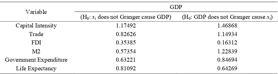
Granger’s causality test was conducted to predict any causality relationship between GDP’s growth and trade, the FDI, and the capital intensity on each country. The results show there is no evidence of causality’s effect from GDP’s growth, or from trade, the FDI, or the capital’s intensity. The FDI exhibits a causality effect on GDP’s growth in Singapore, the Philippines, and Thailand in one direction only. Trade also has a causality effect in one direction in the Philippines and Thailand, while capital intensity indicated a causality effect on GDP’s growth in the Philippines only. The results indicate there are no reverse causality issues. The estimation result of the ECM model for each country is shown in Table A.2 (Appendix).
The ECM term shows the speed of adjustment’s value of economic growth in each country due to changes in the determinant variables. A negative and significant value of ECM indicates that the overall effect is to boost economic growth, thereby forcing economic growth back towards its long run growth path, as determined by the capital intensity, trade, and the foreign direct investment. The fastest adjust-ment to the equilibrium pattern was experienced by the Philippines.
intensity’s growth effect will be very significant if it occurred in developed countries, rather than in developing one.
Trade’s openness in Indonesia and Malaysia shows a negative impact, meanwhile the others experience a positive effect. These results indicate that an open trade economy does not always have a positive impact on growth, particularly when these countries do not have sufficient preparation to anticipate trade’s openness and to maintain the comparative advantage of their export products in the global markets, which results in decreased exports. This analysis is similar to a study by Simorangkir (2006) which used the SVAR model to analyse trade openness’s impacts on the Indonesian economy. Moreover, Daumal and Özyurt (2011) predict that trade openness favors more industrialized states, which are well-endowed in human capital, rather than states whose economic activities are mainly based around agriculture.
However this result is debatable. Its main weakness is that it is mainly from outcome-based measures, and as such, is the result of very complex interactions between numerous factors so that it is not clear what such measures capture exactly. On the other hand, the endogenous growth theory has provided a framework for the positive growth effect of trade through innova-tion’s incentives, technologies diffusion and knowledge’s dissemination. Inspired by these theoretical developments, Hausmann et al. (2007) propose an analytical framework linking the type of goods (as defined in terms of their productivity level) a country specializes in to its rate of economic growth. In order to test empirically for this relationship, they defined an index aiming at capturing the productivity level (or the quality) of at basket of goods exported by each country. Using various panel data estimators during the period from 1962 to 2000, their growth regression showed that countries which exported goods with higher productivity levels (or higher quality goods) had higher growth performances. These results suggest that what countries export does matter, with regards to the growth effect of trade.
Unlike the trade effect, openness in foreign investments, described by the value of the net foreign direct investment gives a similar conclusion. The FDI indicates a positive effect on GDP’s growth in all the countries, however it’s only significant in Malaysia and Singapore. The complementarities between FDI and growth have been well documented in the empirical literature (see, for example, Mencinger, 2003; Lee & Tcha, 2004). Although many studies have confirmed the positive effects of FDI on the host country’s economic growth, some authors stress that there is still no consensus on the degree of these effects (Blomström, M. & Kokko, A. 1998; Lim, E., 2001).
Panel Data Estimation’s Result
A method which can be used is the Autoregressive Distributed Lag (ARDL), a dynamic equation model that incorporates the lag of the dependent variable and the lag of the independent variables as part of the regression. Pesaran et al (1999) examined the use of the ARDL model for long-term relationships’ analysis when the combination of variables are
I(1), and found that the ARDL models have advantages in providing long-term coefficient estimations consistently, regardless of whether the variable’s regression is integrated in I(1) or
I(0).Thenumber of choices for the lags uses Alt and Tinbergen’s approach (Gujarati & Porter, 2009). They suggest that to estimate the ARDL, one may proceed sequentially. This sequential procedure stops when the regression coefficients of the lagged variables start becoming statis-tically insignificant and/or the coefficient of at least one of the variables changes sign from positive to negative or vice versa. The model that was used here is as follows:
+
shows there is no evidence of causality’s effect between GDP’s growth and all the explanatory variables used by both side. However, we cannot ignore endogeneity issues in case of an
unobservable individual-specific effect being included in the error term, which correlates with the explanatory variable. We undertake Chow’s test to demonstrate the influence of individual effects in the model, and compare the OLS model with the fixed effects.This Fixed Effects (FE) least squares, also known as Least Squares Dummy Variables (LSDV), suffer from a large loss of degrees of freedom. Chow’s test is a simple test with the Restricted Residual Sums of Squares (RRSS) being those of the OLS in the pooled model, and the Unrestricted Residual Sums of Squares (URSS) being those of the LSDV’s regression (Baltagi, 2005). The result denotes an insignificant statistic value. This means that as there is no individual specific effect in this model, then the cross section data
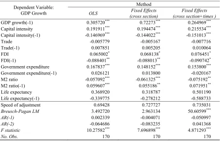
can be pooled. Due to the absence of an individual specific effect, the OLS model can still be an option to provide an efficient and consistent estimation. However, the fixed effects method is also presented. The estimation’s result is shown in Table 1.
The value of the lagged dependent variable is as expected, being in the range 0 < λ <1, which means the short-term dynamic model will converge towards the long-term one. This value relates to the speed of adjustment obtained by (1 -λ). The speed of adjustment of the pooled OLS method is lower than the speed of adjustment resulting from the fixed effect model and the robust least square. As predicted, when imposing the assumption of homogeneity, this will cause a rise in bias in the coefficient of the lagged dependent variable (Pesaran etal., 1998). A speed for the adjustment values of greater than 0.50 indicates if the economic growth in the ASEAN 5 countries has a dynamic movement.
Table 1. Regression Estimation Results Comparison with Pooled OLS and Fixed Effect Method
Dependent Variable: GDP Growth
Method
OLS Fixed Effects (cross section)
Fixed Effects (cross section+times ) GDP growth(-1) 0.305720*** 0.72273*** 0.264969*** Capital intensity 0.191911*** 0.194474*** 0.215534*** Capital intensity(-1) -0.146969*** -0.144022*** -0.151013***
Trade -0.005779 -0.005167 -0.007716
Trade(-1) 0.007851 0.005205 0.010064
FDI 0.065002* 0.068138* 0.076451*
FDI(-1) -0.088401** -0.088013** -0.090742*
Government expenditure 0.167837*** 0.148152*** 0.153800*** Government expenditure(-1) 0.026121 0.013800 -0.020167 M2 ratio -0.057092*** -0.061325*** -0.075192** M2 ratio(-1) 0.059607*** 0.055186** 0.071951**
Life expectancy 0.368920 0.318787 0.501190
Life expectancy(-1) -0.339775 -0.278212 -0.588733
Speed of adjustment 0.69428 0.727727 0.735031
Breusch-Pagan LM 3.492720 2.963134 50.60599***
AR(-1) 0.002339 -0.004071 -0.050997
AR(-2) -0.064686 -0.083235 0.041368
F statistic 10.27582*** 7.696898*** 4.871293***
No. Obs. 170 170 170
All the models support the theory’s predictions. The greater that the value for the capital intensity is, this will encourage a country to experience higher economic growth. Countries with abundant capital will have a high capital intensity and tend to specialize in capital-intensive industries, as predicted by Heckscher-Ohlin. Presumably it makes sense if almost all the countries seek to advance their industrial structures and try to become countries with capital intensive industry’s structures because this would encourage higher economic growth. Countries with a capital-intensive industry’s characteristics are usually developed countries or industrialized countries that have a higher per capita income than the developing countries.
Trade data released by UNComtrade shows if there has been a shift in the trade pattern so the ASEAN countries that began to be exporters of products which are parts for other manufactured products, such as machinery and transport equipment (SITC 7), or manufactured goods classified chiefly by their materials (SITC 6) and miscellaneous manufactured articles (SITC 8).These indicate a changing trend in the pattern of developing countries’ exports, or the types of products being manufactured, in accordance with the different stages of their industriali-zation. Newly industrializing countries, for example, can slowly change their exports towards capital-intensive products, while their position is replaced by another country which is running at a slower industrialization rate, as found by Yeats(1989).
Openness to foreign investment seems to have greater and more significant impact on economic growth than trade openness. So far, foreign investment is needed by developing countries as a form of aid capital to finance their development. The most important is that the FDI can also be a source of new technology, mana-gerial skills and marketing networks. FDI can also provide a stimulus to competition, innovation, savings and capital formation which brings job creation and economic growth.
The significant effect of FDI is unlike the effect of the trade ratio on GDP, which apparently has no significant effect on GDP’s
growth. The classical cross-section empirical study by Levine and Renelt (1992) also cannot offer support for any independent and robust relationship between trade and growth. Sala-i-Martin (1997) and Vamvakidis (2002) also do not find any robust correlation between trade and economic growth. By looking at the historical data from 1870 to the present, Vamvakidis (2002) finds no support for the positive openness-growth link, which appears to be a phenomenon of the recent decades. More recently, Rodriguez (2006) cast serious doubts about the consistency of the trade and growth relationship, which is very sensitive to the countries and time periods selected for the comparison, the measures of openness used as well as the way it is instrumented in the regression analyses. Rodriguez and Rodrik (2001) carried out a systematic critique of pre-vious research findings by demonstrating selection biases in the studies reviewed. By correcting for these shortcomings, the claimed positive relationship disappears. The paper by Rodrik et al. (2004) constitutes a case in which not only the impact of institutions on growth is more relevant than that of openness, but also the coefficient of the trade/GDP ratio turns out to be negative.
Wacziarg and Welch (2003), for example, have evidenced two problematic aspects of this literature: (i) The vast amount of heterogeneity across countries in the regression analysis, (ii) the non-adequacy of a simple dichotomous indicator of openness, to discriminate between slow and fast growing countries. In their work, when the openness dummy is substituted by trade shares, the link between trade and growth becomes negative and insignificant. A study by
structure of trade for the TE. These measures are revealed to be positively and robustly associated with growth.
The finding of a negative correlation for the two major samples studied raises doubts about the importance of this variable on long-run growth’s performance. It is known that the conventional trade theory associates interna-tional trade with a reallocation of resources within the national borders. This reallocation generates efficiency gains that increase the level
of GDP, but there are doubts whether these level effects are temporary or permanent. According to Levine and Renelt (1992); Baldwin and Seghezza (1996), there should be an indirect channel that goes from trade to investment and then growth. An equally likely and plausible explanation is that the standard measures of openness have been adopted. Rather than traditional definitions, a more comprehensive measure of openness can do a better job in detecting growth’s impact (Capolupo & Celi, 2008).
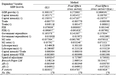
Initial analysis has shown that industrial structures, which are reflected by capital intensity and economic openness, especially in FDI, have a significant effect on economic growth. However, the above analysis shows the effect of each variable by holding the other control variables constant. Next the integration of both existing conditions, the industrial structure and openness, is conducted to see how they affect economic growth. This analysis also intended to provide valid and robust estimations. The results are as shown in Table 2.
The result indicates that capital intensity and trade’s interaction have positive relationship on economic growth, but not so strongly that make a significant impact. This positive relationship shows that open trade can encourage domestic investment, by increasing domestic specialization. Export enhancements should not always have to be followed by the addition of new workers, because there is possibility of labor movement across sectors, as suggested by Heckscher-Ohlin-Samuelson. The movement of
Table 2.Interaction of Capital Intensity and Openness Effects on Growth Estimation Results
Dependent Variable: GDP Growth
Method
OLS Fixed Effects (cross section)
Fixed Effects (cross section+times ) GDP growth(-1) 0.308153*** 0.272003*** 0.2606191*** Capital intensity 0.162171*** 0.162452*** 0.188705*** Capital intensity(-1) -0.150551*** -0.147107*** -0.150755***
Trade -0.005755 -0.005770 -0.008598
Trade(-1) 0.005116 0.001477 0.008012
FDI 0.079039** 0.088083** 0.081340*
FDI(-1) -0.090657** -0.091628** -0.087901*
Government expenditure 0.165378*** 0.141307*** 0.157034*** Government expenditure(-1) 0.031980 0.015975 -0.012695 M2 ratio -0.057304*** -0.061798*** -0.076318** M2 ratio(-1) 0.05792*** 0.053246** 0.071321***
Life expectancy 0.349628 0.301103 0.522859
Life expectancy(-1) -0.296687 -0.213126 -0.553229
Capital intensity*Trade 0.000304 0.000350 0.000256
Capital intensity*FDI -0.002693 -0.003990 -0.001390
Speed of adjustment 0.691847 0.727997 0.739381
Breusch-Pagan LM 3.398224 2.969514 50.53411***
AR(-1) -0.001949 -0.001949 -0.038705
AR(-2) -0.049912 -0.049912 -0.072825
F statistic 8.883852*** 6.914785*** 4.635626***
No. Obs. 170 170 170
labor to the sector that increases its speciali-zation indirectly reduces the costs of hiring labor. Rises in productivity and reductions in production costs contribute to increasing economic growth (Daumal & Özyurt, 2011). Wacziarg and Welch (2008) state how liberalization has fostered growth through its effect on physical capital’s accumulation. The growth enhancing impact of FDI depends critically on the absorptive capacity of a host country and whether FDI crowds out its domestic investment. Absorptive capacity is defined as the measurement that determines a country’s ability to generate and/or absorb FDI spillovers. Previous studies summarized by Farkas (2012) show that the absorptive capacity depends on a minimum threshold level of human capital, well developed financial markets, trade openness, levels of income, and the techno-logical gap. The interaction term estimates the combined impact of FDI and capital intensity on growth and indicates the nature of the relationship between the two (Makki & Somwaru, 2004). A negative coefficient for this interaction term suggests that FDI crowds out domestic investment.
The entry and presence of foreign investors does not only have an impact on the technologies used by domestic firms, but it also affects various other characteristics of the host country’s market (Kokko & Thang, 2014). Apart from their direct and indirect effects on technology choices and knowledge, foreign investors may have some influence on the nature and intensity of competition and on the demand, supply, and quality of inputs and intermediate goods. For example, FDI typically results in an increased competition in both the output markets and the markets for skilled labor and other inputs, which may result in the crowding out of domestic firms. Another rebuttal of the argument that FDI promotes growth comes from Prasad et al. (2007) who posits that non-industrial coun-tries which have relied on foreign capital, have not grown faster than those countries that have not relied on these flows, adding that foreign capital has a greater impact on growth only in the industrial countries. They argue that
developing countries have a limited absorptive capacity for foreign capital inflows because of the existence of weak financial markets, and because these countries are prone to currency over valuations.
Analysis by Kokko (1994) offers some obvious policy conclusions for host country governments that wish to encourage foreign investment in order to benefit from its technology spillovers. Efforts to promote FDI should perhaps focus on industries where local technological capabilities are already relatively strong, or where product differentiation and economies of scale are not so significant that the foreign firms can easily take over the whole market. Lapan and Bardhan (1973) show that technical advances (and technologies) applicable to the factor-proportions of capital-rich developed countries are hardly of any use in improving the techniques of low capital-intensity less developed countries.
Other control variables also provide significant contributions to economic growth. Two types of government policy, namely fiscal policy through the government’s expenditure and monetary through the management of money supply (M2), have significant effects, although in different directions. Greater govern-ment spending will boost economic growth. Meanwhile, the higher the ratio of M2 becomes, will lead to inflation which results in decreased growth. These results are indeed consistent with our predictions.
innovation and of technical change, which propels all the factors of production (Mincer, 1981). A study by Romer (1989) of a regression equation that tries to estimate separate roles for both the physical investment and the human capital variables to explain the rate of output’s growth, finds that collinearity may cause the human capital’s variables not to enter with any great significance. In addition, they should still have an explanatory power for investment. However, this paper does not explore this phenomenon any further.
CONCLUSION
The debate over the effect of economic openness on the growth of a country never finishes. In spite of the wave of liberalization undertaken during the last decades, the debate on the links and causality between openness and growth is still open. Empirical results most often suggest that, in the long run, more outward-oriented countries register better performance in their economic growth. However, this empirical evidence continues to be questioned for at least two main reasons: There are still some discussions and doubts on the way countries’ openness is measured on the one hand, and the debate about the estimation’s methodology is still open on the other hand.
Using data of the ASEAN 5 countries, both the time series and panel data confirm the effect of trade openness and international capital flows are not always positive. The domestic charac-teristic that consistently gives a positive effect is a country’s capital intensity. This variable can be seen as a comparative advantage belonging to a country and leading to its industrial structure. The higher the capital intensity a country has means the more capital-intensive its industries can be. Higher capital intensity significantly increases economic growth in all the models.
Solving an endogeneity issue, we apply a fixed effects method to control the time invariant unobservable variables which can lead to bias. However, these fixed effects still cannot fix the autocorrelation and heteroscedasticity problems. In such cases, we employ a three steps feasible least square method in order to get unbiased and
consistent estimations. The interaction estima-tion between capital intensity and openness, both for trade and foreign direct investment, gives similar results of an insignificant effect of both interaction variables on economic growth. These insignificant effects show there is no evidence that an open capital-intensive country expe-riences higher economic growth than other countries do. Overall the results still leave questions about the appropriate indicators for openness, especially for measuring trade’s liberalization, and what channel it uses to effect economic growth. These become our study limitations that can be the focus for exploration in a new study.
REFERENCES
Acemoglu, D., & Guerrieri. (2008). Capital Deepepening and Nonbalance Economic Growth. Journal of Political Economy, Vo. 116, No. 3 , 467-498.
Ashraf, Q. H., Lester, A., & Weil, D. N. (2008).
When Does Improving Health Raise GDP?
NBER Working Paper No. 14449.
Bailliu, J. N. (2000). Private Capital Flows, Financial Development,and Economic Growth in Developing Countries. Bank of Canada.
Baldwin, R., & Seghezza, E. (1996). Testing for Trade-Induced Investment-Led Growth.
NBER Working Paper 5416.
Baltagi, B. H. (2005). Econometric Analysis of Panel Data. West Sussex: John Wiley & Sons Ltd.
Barro, F., & Sala-i-Martin, X. (2004). Economic Growth. Cambridge: MIT Press.
Barro, R. (1991). Economic Growth in a Cross Section of Countries. The Quarterly Journal of Economics, Vol. 106, No. 2 , 407-443. Berlemann, M., & Wesselhöft, J.-E. (2012).
Estimating Aggregate Capital Stocks Using the Perpetual Inventory Method – New Empirical Evidence for 103 Countries –.
Hamburg: Department of Economics Helmut Schmidt University.
Blomström, M., & Kokko, A. (1998). Multinational Corporations and Spillovers.
Braun, M., & Raddatz, C. (2007). Trade liberalization, Capital Account Liberali-zation and the Real Effects of Financial Development. UC Santa Cruz conference.
Capolupo, R., & Celi, G. (2008). Openness and Economic Growth: A Comparative Study of Alternatif Trading Regimes . Economie Internationale, No. 116 , 5-35.
Caporale, G. M., & Girardi, A. (2012). Business Cycles, International Trade and Capital Flows Evidence from Latin America. Berlin: Deutsches Institut für Wirtschaftsforschung. Cipollina, M., Giovannetti, G., Pietrovito, F., &
Pozzolo, A. F. (2011). FDI and Growth: What Cross-Country Industry Data Say.
Economics & Statistics Discussion Paper No. 060/11, Università degli Studi del Molise.
Daumal, M., & Özyurt, Ö. (2011). The Impact of International Trade Flows on Economic Growth in Brazilian States. Review of Economics and Institutions, Vol. 2, No.1 . Edwards, S. (March 1997). Openness,
Productivity and Growth: What We Really Know? NBER Working Paper No.5978 . Edwards, S. (1993). Trade Policy, Exchange
Rates, and Growth. NBER Working Paper No. 4511 .
Farkas, B. (2012). Absorptive Capacities and the Impact of FDI on Economic Growth.
Deutsches Institut für Wirtschaftsforschung Discussion Paper No. 1202 .
Gujarati, D. N., & Porter, D. C. (2009). Basic Econometrics. New York: McGraw-Hill/Irwin.
Gundlach, E. (1997). Openness and Economic Growth in Developing Countries.
Weltwirtschaftliches Archiv Vol. 133, Iss. 3 , 479-496.
H., L., & P., B. (1973). Localized Technical Progress and Transfer of Technology and Economic Development. Journal of Econo-mic Theory, Vol. 6 , 585-595.
Hall, R. E., & Jones, C. I. (1999). Why Do Some Countries Produce So Much More Output Per Worker Than Others? The Quarterly Journal of Economics, Vol. 114, No. 1 , 83-116.
Harris, R. (1995). Using Cointegration Analysis in Econometric Modelling. Prentice Hall.
Hausmann, R., Hwang, J., & Rodrik, D. (2007). What You Export Matters. J Econ Growth, Vol. 12 , 1-25.
Henry, P. B. (2003). Capital Account Libera-lization, The Cost of Capital, and Economic Growth. NBER Working Paper No. 9488 . Inklaar, R., & Timmer, M. P. (2013). Capital,
Labor and TFP in PWT 8.0. Groningen Growth and Development Centre, Univer-sity of Groningen.
Insukindro, & Sahadewo, G. A. (2010). Inflation Dynamics in Indonesia: Equilibrium Correction and Forward-Looking Phillips Curve Approaches. Gadjah Mada Inter-national Journal of Business, Vol. 12, No. 1
, 117-133.
Jin, K. (2012). Industrial Structure and Capital Flows. The American Economic Review, No. 102(5) , 2111-2146.
Kawai, M., & Wignaraja, G. (2014). Trade Policy and Growth in Asia. Tokyo: Asian Development Bank Institute.
Kokko, A. (1994). Technology, Market Characteristics, and Spillovers. Journal of Development Economics, Vol. 43 , 279- 293. Kokko, A., & Thang, T. T. (2014). Foreign
Direct Investment and the Survival of Domestic Private Firms in Viet Nam. Asian Development Review, vol. 31, no. 1 , 53–91. Lawrence, R. Z., & Weinstein, D. E. (1999).
Trade and Growth: Import - Led or Export - Led? Evidence from Japan and Korea.
Cambridge: NBER Working Paper 7264. Lee, M., & Tcha, M. (2004). The Color of
Money: The Effects of Foreign Direct Investment on Economic Growth in Transition Economies . Review of World Economies, Vol. 140, No. 2 , 211-229. Levine, R., & Renelt, D. (1992). A Sensitive
Analysis of Cross-Country Growth Regressions. American Economic Review, No. 82 , 942-963.
Lim, E. (2001). Determinants of, and the Relation Between, Foreign Direct Invest-ment and Growth: A Summary of the Recent Literature. International Monetary Fund Working Paper.
Lim, G., & McNelis, P. D. (2014). Income Inequality, Trade and Financial Openness.
Challenges Facing. Washington: Interna-tional Monetary Fund.
Lin, J. Y. (2003). Development Strategy. Viability, and Economic Convergence.
Economic Development and Cultural Change, Vol. 51, No. 2 , 277-308.
Lin, J. Y., & Zhang, P. (2009). Industrial Structure, Appropriate Technology and Economic Growth in Less Developed Countries. Policy Research Working Paper No. 4905, The World Bank .
Makki, S. S., & Somwaru, A. (2004). Impact of Foreign Direct Investment and Trade on Economic Growth: Evidence from Developing Countries. American Journal of Agricultural Economics, vol. 86, issue 3 , 795-801.
Medvedev, D. (2006). The Impact of Preferen-tial Trade Agreements on Foreign Direct Investment Inflows. World Bank Policy Research Working Paper No. 4065.
Mencinger, J. (2003). Does Foreign Direct Investment Always Enhance Economic Growth? Kilkos, Vol. 56, No. 4 , 491-508. Mincer, J. (1981). Human Capital and Economic
Growth . Cambridge: NBER Working Paper No. 803.
Nelson, R. R., & Pack, H. (1999). The Asian Miracle and Modern Growth Theory. The Economic Journal, Vol. 109, No. 457 , 416-436.
Nowak, F. L. (2000). Trade Policy and Its Impact on Economic Growth: Can Openness Speed Up Output Growth? IAI. Pagan, A. R., & Wickens, M. (1989). A Survey
of Some Recent Econometric Methods. The Economic Journal,Vol. 99, No. 398 , 962-1025.
Park, D., Park, I., & Estrada, G. E. (2008). Prospects of an ASEAN-People's Republic of China Free Trade Area: A Qualitative and Quantitative Analysis. ADB Working Paper Series, No. 130 .
Pesaran, M. H., & Shin, Y. (1999). An Autoregressive Distributed Lag Modelling Approach to Cointegration Analysis. In S. S, Econometrics and Economic Theory in the 20th Century: The Ragnar Frisch Centennial Symposium (p. Ch. 11). Cambridge: Cambridge University Press.
Pesaran, M. H., Shin, Y., & Smith, R. P. (2001). Bounds Testing Approaches to the Analysis of Level Relationship. Journal of Applied Econometrics, Vol. 16 , 289-326.
Pesaran, M. H., Shin, Y., & Smith, R. P. (1998).
Pooled Mean Group Estimation of Long Run Relationships in Dynamic Hetero-genous Panel.
Prasad, E. S. (n.d.). Foreign Capital and Econo-mic Growth. National Bureau of Economic Research .
Rodriguez, F. (2006). Openness and Growth: What Have We Learned? United Nations. Rodriguez, F., & Rodrik, D. (2001). Trade
Policy and Economic Growth: A Skeptic's Guide to the Cross-National Evidence. In B. S. Rogoff, NBER Macroeconomics Annual 2000, Volume 15 (pp. 261 - 338). MIT PRess.
Rodrik, D. (1999). The New Global Economy and Developing Countries: Making Openness Work. Washington: Policy Essay 24, Overseas Development Council.
Rodrik, D., Subramanian, A., & Trebbi, F. (2004). Institutions Rule: The Primacy Over Geography and Interaction in Economic Development. Journal of Economic Growth, Vol. 9 , 131-165.
Romer, P. M. (1989). Human Capital and Growth: Theory and Evidence. Cambridge: NBER Working Paper No. 3173.
Sachs, J. D., & Warner, A. (1995). Economic Reform and the Process of Global Integration. Brookings Papers on Economic Activity .
Sala-i-Martin, X. (1997). I Just Run Two Million Regressions. American Economic Review, Vol. 87, No. 2, Conference and Proceeding, (pp. 178-83.).
Sarel, M. (1996). Growth in East Asia What We Can and What We Cannot Infer.
Washington D.C: International Monetary Fund.
Shiino, K. (2012). Overview of Trade
Agreements in Asia. In Cause and
Consequence of Firm FTA Utilization in Asia. Bangkok: Bangkok Reseach Center, IDE-JETRO.
International Trade and Commodities Study Series No. 44. United Nations Conference on Trade and Development (UNCTD). United, N. (2006). Banking Sector Lending
Behaviour and Efficiency in Selected SECWA Member Countries. United Nations. Vamvakidis, A. (2002). How Robust is the
Growth-Openness Connection: Historical Evidence. Journal of Economic Growth, Vol. 7 , 57-80.
Ventura, J. (1997). Growth and Interdependence.
The Quarterly Journal of Economics , 57-84.
Wacziarg, R., & Welch, K. H. (2003). Trade Liberalization and Growth: New Evidence.
NBER Working Paper No. 10152.
Wacziarg, R., & Welch, K. (2003). Integration and Growth: An Update. NBER Working Paper 10152.
Wacziarg, R., & Welch, K. (2008). Trade Liberalization and Growth: New Evidence.
The World Bank Economic Review, Vol. 22, No. 2 , 187-231.
Winters, A. N., & McKay, A. (2004). Trade Liberaliztion and Poverty: The Evidence So Far. Journal of Economic Literature, Vol. 42 , 72-115.
Wooldridge, J. M. (2005). Introductory Econo-metrics: A Modern Approach. South Western.
Yeats, A. J. (1989). Shifting Patterns of Comparative Advantage: Manufactured Exports of Developing Countries. Working Paper Series No. 165, The World Bank. Yue, C. S. (2004). ASEAN-China Free Trade
APPENDIX
Table A.1. Unit Root Test Results
Variable GDP Growth
Capital
Intensity Trade FDI M2 Ratio
Government Expenditure
Growth
Life Expectancy
ADF-Fisher
Level 47.0790*** 41.9710*** 29.5825*** 10.8845 15.6724 50.6727*** 6.82123 1st diff. 105.283*** 78.4429*** 68.5712*** 97.1508*** 80.9875*** 120.589*** 57.3055*** IPS
Level -5.3090*** -4.6307*** -2.8687*** -0.59784 -1.58417 -5.54743*** 1.09330 1st diff. -10.926*** -8.3803*** -7.5051*** -10.316*** -8.7459*** -12.7748*** -10.9536***
LLC
Level -5.3090*** -5.0656*** -2.5766*** -0.62807 -0.82856 -3.34124*** -0.28793 1st diff. -7.2255*** -7.6249** -8.9555*** -7.5201*** -9.8897*** -11.4128*** -2.46172***
Optimum Lag Length 1 1 1 1 1 1 1
Note: H0: ρ=0 (There are root units, the variable X is not stationary). Sign *** means significant at α = 1%, ** significant at
α = 5%, and * significant at α = 10%.
Table A.2. ECM Model Estimation Results
Country Variables
Capital intensity Trade FDI ECM term Indonesia 0.160107** -0.268194*** 0.177857 -0.662445*** Malaysia 0.218878*** -0.015294 0.844416*** -0.845240*** Philippines 0.280787*** 0.088185 0.049269 -0.908787*** Singapore 0.276071*** 0.063573** 0.167422*** -0.878276*** Thailand 0.296608*** 0.044688 0.001745 -0.878855*** Sign *** means significant at α = 1%, ** significant at α = 5%, and * significant at α = 10%, number of observations: 35.
Table A.3. Granger Causality Estimation Results
Variable GDP
(H0: xi does not Granger cause GDP) (H0: GDP does not Granger cause xi)
Capital Intensity 1.17492 1.46868
Trade 0.82626 1.14934
FDI 0.35385 0.16312
M2 0.57354 1.22839
Government Expenditure 0.63221 0.84694
Life Expectancy 0.81092 0.64269
Note: no values are significant