Full Terms & Conditions of access and use can be found at
http://www.tandfonline.com/action/journalInformation?journalCode=ubes20
Download by: [Universitas Maritim Raja Ali Haji] Date: 12 January 2016, At: 23:56
Journal of Business & Economic Statistics
ISSN: 0735-0015 (Print) 1537-2707 (Online) Journal homepage: http://www.tandfonline.com/loi/ubes20
Powerful Trend Function Tests That Are Robust to
Strong Serial Correlation, With an Application to
the Prebisch–Singer Hypothesis
Helle Bunzel & Timothy J Vogelsang
To cite this article: Helle Bunzel & Timothy J Vogelsang (2005) Powerful Trend
Function Tests That Are Robust to Strong Serial Correlation, With an Application to the Prebisch–Singer Hypothesis, Journal of Business & Economic Statistics, 23:4, 381-394, DOI: 10.1198/073500104000000631
To link to this article: http://dx.doi.org/10.1198/073500104000000631
Published online: 01 Jan 2012.
Submit your article to this journal
Article views: 82
View related articles
Powerful Trend Function Tests That Are Robust
to Strong Serial Correlation, With an Application
to the Prebisch–Singer Hypothesis
Helle B
UNZELDepartment of Economics, Iowa State University, Ames, IA 50011-1070 (hbunzel@iastate.edu)
Timothy J. V
OGELSANGDepartment of Economics, Cornell University, Ithaca, NY 14853-7601 (tjv2@cornell.edu)
We propose tests for hypotheses on the parameters of the deterministic trend function of a univariate time series. The tests do not require knowledge of the form of serial correlation in the data, and they are robust to strong serial correlation. The data can contain a unit root and still have the correct size asymptotically. The tests that we analyze are standard heteroscedasticity autocorrelation robust tests based on nonpara-metric kernel variance estimators. We analyze these tests using the fixed-basymptotic framework recently proposed by Kiefer and Vogelsang. This analysis allows us to analyze the power properties of the tests with regard to bandwidth and kernel choices. Our analysis shows that among popular kernels, specific kernel and bandwidth choices deliver tests with maximal power within a specific class of tests. Based on the theoretical results, we propose a data-dependent bandwidth rule that maximizes integrated power. Our recommended test is shown to have power that dominates a related test proposed by Vogelsang. We apply the recommended test to the logarithm of a net barter terms of trade series and we find that this series has a statistically significant negative slope. This finding is consistent with the well-known Prebisch–Singer hypothesis.
KEY WORDS: Data-dependent bandwidth; Deterministic trend; Fixed-basymptotics; Heteroscedastic-ity autocorrelation estimator; Linear trend; Nearly integrated; Partial sum; Power enve-lope; Unit root.
1. INTRODUCTION
In this article we propose tests of linear hypotheses on the parameters in a univariate deterministic trend model. The tests are designed to be size-robust to strong serial correlation in the errors, including the case of a unit root in the errors. Robustness to serial correlation is obtained using well-known nonpara-metric heteroscedasticity autocorrelation (HAC) robust stan-dard errors. Tests using the HAC robust stanstan-dard errors may still have significant size distortion, however. One source of this distortion is the fact that the finite-sample distributions of HAC robust tests are highly dependent on the choice of band-width and kernel, whereas the asymptotic distributions of the tests do not depend on these choices. Using the newly de-veloped fixed-bandwidth (fixed-b) asymptotics of Kiefer and Vogelsang (2002), we develop an asymptotic theory that cap-tures the choice of kernel and bandwidth. Fixed-basymptotics can be used to reduce some of the size distortions. The sec-ond source of size distortion is the possibility of strong serial correlation (possibly a unit root) in the errors. We show that the fixed-basymptotic distributions are free of serial correlation nuisance parameters regardless of the bandwidth or kernel used to compute the HAC robust standard errors. This asymptotic pivotal result holds for stationary errors as well as nearly in-tegrated errors, although the limiting distributions are different in the two cases. Using this asymptotically pivotal property, we are able to control the overrejection problem caused by strong serial correlation by implementing the scaling correction ap-proach proposed by Vogelsang (1998). Therefore, the tests that we propose have well-behaved size even when the errors have strong serial correlation.
For the special case of the simple linear trend model, we use a local asymptotic power analysis to guide the choice of kernel and bandwidth. Confining attention to tests with asymptotically correct size, we consider a class of well-known and popular kernels and compute asymptotic power envelopes that repre-sent maximal power across the kernels and bandwidths within the class. We then show that tests based on the Daniell kernel have power that effectively attains the power envelope. We ad-dress the traditionally difficult issue of HAC bandwidth choice using fixed-b asymptotics in conjunction with local to unity asymptotics. For a given value of the local to unity parame-ter, we numerically determine the bandwidth that maximizes integrated power. To our knowledge, this is the first detailed HAC bandwidth analysis that focuses on the power of tests rather than on the mean squared error of the HAC estimate, al-though Hall (2004) pointed out a potential link between band-width choice and the power of overidentifying restrictions tests in generalized method-of-moments models. Our analysis pro-vides a data-dependent bandwidth that maximizes integrated power. Finite-sample simulations suggest that a feasible version of this data-dependent bandwidth rule works well in practice. Our asymptotic and finite-sample analysis points to one HAC-based test that we recommend in practice.
We compare our recommended test with the related tests pro-posed by Vogelsang (1998). One of those tests, thet-PSWtest, is very similar to the tests analyzed in this article. We show that
© 2005 American Statistical Association Journal of Business & Economic Statistics October 2005, Vol. 23, No. 4 DOI 10.1198/073500104000000631 381
the t-PSW test is dominated in terms of power by the recom-mended test. Therefore, the tests analyzed in this article are an improvement over the tests proposed by Vogelsang (1998).
We use the recommended test to investigate the well-known Prebisch (1950) and Singer (1950) hypothesis postulating that over time, the net barter terms of trade should be declin-ing between countries that primarily export commodities and countries that primarily export manufactured goods. This em-pirical conjecture has received considerable attention in the in-ternational economics literature (see, e.g., Ardeni and Wright 1992; Cuddington and Urzua 1989; Grilli and Yang 1988; Lutz 1999; Powell 1991; Sapsford 1985; Spraos 1980; Trivedi 1995). The empirical results in the literature have been mixed. Many authors have interpreted evidence in support of the Prebisch– Singer hypothesis with caution because of the potential over-rejection problem caused by strong serial correlation/unit root in the errors. In fact, many authors have focused on, and in our opinion been distracted by, the question as to whether or not the innovations have a unit root or are stationary. Because a time series can have a decreasing deterministic trend whether the in-novations are stationary or have a unit root, the unit root issue is simply a nuisance parameter in the context of the Prebisch– Singer hypothesis. One advantage of our approach is that it al-lows a direct test on the slope coefficient of the linear trend that is robust to the unit root question. When applied to the net barter terms of trade series of Grilli and Yang (1988) as extended by Lutz (1999) we find strong and consistent evidence to support the Prebisch–Singer hypothesis. Our results are not subject to the usual “overrejection problem” critique because of the ro-bust properties of the tests. Further tests indicate that the trend function of this series is stable over time. Our results confirm what many authors have been saying for more than 20 years: Prebisch and Singer were right!
The rest of the article is organized as follows. Section 2 de-scribes the trend function model in detail, states the required assumptions, and presents some of the basic asymptotic results. Section 3 describes the scaling procedure used to control the overrejection problem caused by strong serial correlation. Sec-tion 4 briefly describes thet-PSW test proposed by Vogelsang (1998). Section 5 derives and discusses asymptotic results ob-tained under the new fixed-basymptotics. Section 6 examines the asymptotic properties of the test statistics in the simple linear trend model. We compute asymptotic power envelopes, and determine kernels and bandwidths that deliver tests with power close to the envelopes. Section 7 proposes a feasible data-dependent bandwidth rule that builds on the theoretical re-sults, and Section 8 reports the results of some finite-sample simulation experiments. Section 9 gives the empirical results on the Prebisch–Singer hypothesis. Section 10 concludes. Appen-dix A gives proofs of important results, and AppenAppen-dix B gives the formulas for the kernels used.
2. MODEL SETUP
We are interested in the following model of a time series with deterministic trends:
yt=f(t)′β+ut, t=1, . . . ,T, (1) wheref(t)denotes a(k×1)vector of trend functions,β is a
(k×1)vector of parameters, and “′” denotes the transpose,
when used in the context of a vector. This type of model is used frequently in macroeconomics and finance to determine the composition of univariate time series. When performing tests onβ(e.g., to determine whether a given trend should be included), the presence of serial correlation and heteroscedas-ticity in the errors must be taken into account. In this article we concern ourselves with the situation where the exact error structure is not of interest. In that case there is no need to model the error structure explicitly, because hypotheses on the coeffi-cients on the trends can be tested without doing so. Such testing is virtually always done using HAC estimators to estimate the asymptotic variance of the parameter estimates, and we follow that approach in this article.
Throughout the article, we assume thatutis a scalar, mean-0 time series. The time series process{ut}is allowed to have ser-ial correlation and may be stationary or have a unit root or a root close to 1. For the purpose of studying the impact of these vari-ous error specifications on the testing procedures, we make the following flexible assumption aboutut.
Assumption 1.
ut=αut−1+εt, t=2,3, . . . ,T, u1=ε1,
εt=d(L)et, d(L)= ∞
i=0
diLi, ∞
i=0
i|di|<∞,
d(1)2>0,
where{et}is a martingale difference sequence withE(e2t|et−1,
et−2, . . . )=1 and suptE(e4t) <∞. Under this specification, the errors are stationary when|α|<1. In this caseαis not modeled as a function of the sample size. Alternatively, the errors can be modeled as nearly integrated by lettingα=(1−αT), where
α=0 corresponds to a pure unit root process.
Under Assumption 1, the following functional central limit theorems follow from well-known results (see Chan and Wei 1988; Phillips 1987; Phillips and Solo 1992):
T−1/2
[rT]
t=1
ut⇒σw(r) if|α|<1
and
T−1/2u[rT]⇒d(1)Vα(r) ifα=1−
α
T,
whereσ2=d(1)2/(1−α)2,w(r)is a standard Wiener process,
Vα(r)=
r
0exp(−α(r−s))dw(s), ⇒ denotes weak
conver-gence, and[rT]is the integer part ofrTwithr∈ [0,1]. At times it will be useful to stack the data in (1) and rewrite the model as
y=f(T)β+u. (2)
Here f(T) is the (T ×k) stacked vector of trend functions. The following assumption on the trend is sufficient to obtain the main results of the article.
Assumption 2. f(t)includes a constant, there exists a(k×k)
diagonal matrix τT and a vector of functions F, such that
τTf(t)=F(Tt)+o(1),
1
0Fi(r)dr <∞, i = 1, . . . ,k, and
det[01F(r)F(r)′dr]>0.
Assumption 2 is fairly standard and is essentially the same as the assumption used by Vogelsang (1998). We include the additional assumption that an intercept is included in the model. Model (1) is estimated using ordinary least squares (OLS), andβ=(f(T)′f(T))−1f(T)′ydenotes the OLS estimate of β, whereasu=y−f(T)βdenotes the OLS residuals. The limiting distribution ofβis well known for both stationary and unit root errors,
T1/2τ−T1(β−β)⇒σ
1
0
F(r)F(r)′dr
−1 1
0
F(r)dw(r)
if|α|<1
and
T−1/2τ−T1(β−β)
⇒d(1)
1
0
F(r)F(r)′dr
−1 1
0
F(r)Vα(r)dr
ifα=1−α T.
Notice that when the errors are stationary, the only unknown nuisance parameter in the limiting distribution isσ. A single nuisance parameter appears in the limiting distribution of the OLS estimates because the regressors are deterministic. In a re-gression model with random regressors, the asymptotic vari-ance of the OLS estimates depends on a zero-frequency spectral density matrix with rank equal to the number of regression pa-rameters. In that case, the HAC robust standard errors are com-puted using a vector of time series comprising of products of the regressors and OLS residuals.
When the errors are nearly integrated, the only unknown nui-sance parameters ared(1)andα. The dependence of the tests on α when the errors are nearly integrated is the reason that HAC robust tests tend to be oversized in practice when errors have strong serial correlation.
An estimator ofσ2is often used to construct the usual HAC robusttor Wald tests. We consider the case where σ2is esti-mated nonparametrically using the OLS residuals,ut,
σ2=γ0+2 T−1
j=1
k(j/M)γj, (3)
whereγj=T−1Tt=j+1utut−jandk(x)is a kernel function sat-isfying k(x)=k(−x), k(0)=1, |k(x)| ≤1, k(x) continuous at x=0 and 01k2(x)dx<∞. M is called “the bandwidth” or the “truncation lag.” Forσ2 to be consistent, it is neces-sary to downweight or eliminate the sample autocovariances for high values ofj. Specifically, it is necessary thatM→ ∞and
M/T→0 asT→ ∞. Most commonly used kernel functions have the property that k(x)=0 for |x|>1, effectively elim-inating the sample autocovariances for all values of j greater thanM, inspiring the term “truncation lag.”
We are interested in testing hypotheses of the form
H0:Rβ=d, where R is a q×kmatrix of known constants, dis aq×1 vector of known constants, andq≤k. Typically, R is a matrix selecting single entries of β and d is a vector of 0’s, but we maintain the hypothesis in its general form. As
a rule, the test statistics used to test this type of hypothesis on the trend function are eithertor Wald statistics of the form
W=(Rβ−d)′σ2R(f(T)′f(T))−1R′ −1(Rβ−d)
and
t= R1β−d
σ2R
1(f(T)′f(T))−1R′1 ,
where the subscript in R1 signifies that the restriction matrix
is a vector in the case of the t-test. If the errors are stationary andσ2is a consistent estimator, then thet-test has a standard normal limiting distribution andW has a limiting chi-squared distribution. Unfortunately, when there is strong serial correla-tion in the errors, these standard asymptotic approximacorrela-tions are often inaccurate, and the tests suffer from severe overrejection problems (see Vogelsang 1998, table I). In addition, the finite-sample behavior of the tests are sensitive to the choice of band-width and kernel, yet the standard asymptotics are the same regardless of the kernel or bandwidth. We address both of these issues. We control the overrejection problem using a scaling factor proposed by Vogelsang (1998), and address the band-width and kernel problem by deriving the limiting distributions of the scaled tests under the fixed-basymptotic framework pro-posed by Kiefer and Vogelsang (2002).
3. SCALED STATISTICS
We now describe the scaling procedure proposed by Vogelsang (1998) and introduce a new variant of the approach. The basic idea is to multiplicatively scale thetandW tests by a factor that converges to 1 when the errors are stationary but converges to a nuisance parameter-free random variable when the errors have a unit root. We consider two scaling factors based on two unit root tests. LetJdenote the unit root test pro-posed by Park (1990) and Park and Choi (1988). Consider the regression
yt=f(t)′β+
9
i=p
αiti+ut, (4)
wheretp−1is the highest-order polynomial oftincluded inf(t). Then theJstatistic is defined as
J=SSR(1)−SSR(4) SSR(4)
,
whereSSR(4)is the sum of squared residuals obtained from the estimation of (4) by OLS andSSR(1)is the sum of squared resid-uals from the OLS estimation of (1). The second unit root test is the test proposed by Breitung (2002), defined as
BG=T
−2T t=1St2
SSR(1)
,
whereSt=tj=1uj are the partial sums of the OLS residuals from model (1). Both the J andBGstatistics share the prop-erty of converging to 0 when the errors are stationary. When the errors are nearly integrated, the asymptotic distributions of
JandBGare nondegenerate and depend onα, but otherwise do not depend on nuisance parameters such asd(1).
LetURgenerically denote eitherJ orBG, and letcdenote a constant. The scaling factor
exp(−cUR)
converges to a well-defined random variable when the errors have a unit root but converges to 1 when the errors are station-ary. Using the scaling factor, we now redefine thetandW sta-tistics as
The limiting distributions of t andW are unaffected by scal-ing when the errors are stationary. When the errors are nearly integrated, the scaling factor affects the limiting distribu-tion. Given α, for a specific percentage point, it is pos-sible to compute the constant c such that the asymptotic critical values of each statistic are the same for stationary errors and nearly integrated errors. We follow Vogelsang (1998) and compute c for the case where α=0. By mak-ing the asymptotic critical values the same for stationary errors and unit root errors, the scaling factors solve the over-rejection problem caused by strong serial correlation in the errors.
We use the versions of the statistics given by (5) throughout the remainder of this article. Note that the value of cused in practice depends on the significance level of the test and on the unit root statistic used for the scaling factor. A detailed discus-sion of the choice ofcfor the simple linear trend model is given in Section 6.
4. COMPARISONS TO THEPSW TEST
The HAC robust tests defined by (5) are very closely related to thePSWandt-PSWtests proposed by Vogelsang (1998). The
PSW andt-PSW tests are defined in the same manner, except thatσ2is replaced byT−1s2z, wheres2zis the OLS error variance
is, from the regression obtained by computing the partial sums of regression (1). Tedious algebra can be used to show that
T−1s2z is closely related to the Bartlett kernel estimator of σ2
using residualsut=yt−f(t)′β, whereβ is the OLS estimate from (6). Therefore,T−1s2zis of the same stochastic order asσ2. In the case of the simple linear regression model (see Sec. 6), we compare the asymptotic size and power of thet-PSW test and show that it is dominated by the Daniel kernel HAC robust test. Details are given in Section 6.
Vogelsang (1998) also proposed a second test, labeledt-PS, based on the OLS estimates of regression (6). We do not provide
comparisons to thet-PStest here, given that thet-PSWtest has higher power than thet-PStest when the errors are stationary.
5. LIMITING DISTRIBUTIONS UNDER FIXED-bASYMPTOTICS
In this section we provide the limiting null distributions of
tandW as defined in (5) under the assumption thatM=bT, whereb∈(0,1]. This asymptotic nesting for the bandwidth was proposed by Kiefer and Vogelsang (2002), and results were ob-tained for stationary models estimated by generalized method of moments. The results of Kiefer and Vogelsang (2002) do not apply to parameters associated with deterministic trends or to models with errors that contain unit roots. Therefore, the results given here are new.
Before we proceed, some additional notation and defini-tions are required. As is well known, estimators of coefficients on different trends often converge at different rates. Specifi-cally, the coefficients entering the constraint that converge the slowest will dominate the asymptotic distribution. To formal-ize this, let µi be the largest nonpositive power of time,t, in the non-0 elements in the ith row of RτT. Then define the
q×qdiagonal matrixAin such a way thatAii=Tµi,and let R∗=limT
→∞A−1RτT. In the case, whenq=1, we use R∗1 to denote R∗. Under fixed-b asymptotics, the limiting distri-butions depend on the type of kernel used in computingσ2. The following definition describes the types of kernel that we analyze.
Definition 1. A kernel is labeled as type 1 ifk(x) is twice continuously differentiable everywhere and as type 2 ifk(x)is continuous,k(x)=0 for|x| ≥1 andk(x)is twice continuously differentiable everywhere except at|x| =1.
In addition to kernels that fall in these two categories, we con-sider the Bartlett kernel (which is neither type 1 nor type 2) separately.
The limiting distributions are expressed in terms of the fol-lowing functions and random variables.
Definition 2.
k∗−′ is the first derivative ofk∗from below,
In the case of nearly integrated errors, the limiting distrib-utions of the tests depend on the limiting distribdistrib-utions of the unit root tests used in the scaling factors. LetVα(r)denote the residuals from the projection ofVα(r)onto the space spanned byF(r), and letVα∗(r)denote the residuals from the projection of Vα(r)onto the space spanned by(F(r)′,rp,rp+1, . . . ,r9)′. The following lemma follows directly from Park (1990), Park and Choi (1988), and Breitung (2002).
Lemma 1. Suppose that Assumptions 1 and 2 hold. If
|α|<1, then, asT→ ∞,J⇒0, andBG⇒0. Ifα=1−αT,
We generically denote these limiting distributions byUR∞ in what follows. We can now state the main theorem.
Theorem 1. LetM=bT,b∈(0,1]. Then, under
Assump-Theorem 1 demonstrates that pivotal test statistics are ob-tained under fixed-basymptotics regardless of kernel or band-width, although the limiting distributions of the test statistics depend on the choice of kernel and bandwidth. The limiting
distributions are clearly different when the errors are station-ary and when the errors are nearly integrated. For each com-bination of kernel, bandwidth, scaling factor, and percentage point,ccan be chosen so that the critical values are the same for both stationary errors and unit root errors (α=0). The critical values corresponding to the asymptotic distributions in Theo-rem 1 along with the values ofcare simple to compute numer-ically. A power analysis in the next section indicates specific kernels and bandwidth values that lead to tests with optimal power properties in a model with a simple linear trend. Critical values and details of their computation are given for the recom-mended tests in the simple linear trend model after a discussion of power.
6. OPTIMAL KERNELS AND BANDWIDTHS IN THE SIMPLE LINEAR TREND MODEL
In this section we provide extensive analysis of local asymp-totic size and power of the simple linear trend model. We focus on tests of the slope parameter and derive limiting distributions under a local alternative. This allows us to compute local as-ymptotic power for a wide range of kernels and bandwidths. Because size is well controlled, we base the choice of kernel and bandwidth on how they affect power.
The simple linear trend model is given by
yt=β1+β2t+ut, t=1, . . . ,T. (7) The null hypothesis under consideration is H0:β2≤β0. The
alternative is given by
HA:β2=β0+δg(T),
whereg(T)=T−3/2if|α|<1 andg(T)=T−1/2ifα=1−αT. Thetstatistic for this test is given by
t=
The limiting null distribution oftfollows from Theorem 1. Note thatσ2,J, andBGare exactly invariant (invariant for allT) to the true value ofβ2and hence are exactly invariant to the value ofδ. Therefore, onlyβ2−β0depends on the local alternative.
The following theorem gives the limiting distribution oftunder the local alternative. Using the results of this theorem, it is easy to simulate as-ymptotic power of the t-statistic for different choices of ker-nels and bandwidths. The first step is to simulate asymptotic critical values under the null hypothesis. We did this using 50,000 replications. For each replication, we approximated the Wiener processes implicit in the limiting distributions using
normalized partial sums of 1,000 iid N(0,1) random devi-ates. We focused on five well-known kernels—Bartlett, Parzen, Bohman, Daniell, and quadratic spectral (QS)—the formulas for which are given in Appendix B. We considered the grid of bandwidths given by b=.02, .04, . . . ,1. Given a percent-age point, for a given bandwidth and kernel, we computed val-ues ofcsuch that the asymptotic critical values are the same for |α|<1 andα=1. These values ofcare different for the
JandBGscaling factors. Given the values ofcand the critical values, the second step is to compute rejection probabilities for a grid of values ofνusing simulation methods, thus producing asymptotic power curves.
To guide the choice of kernel and bandwidth, we com-puted power for the five kernels and the bandwidth grid for a grid of values of ν. These calculations were done for
α=0,1,2, . . . ,49,50. For a given value of α and for each value ofν, maximal power across the kernels, bandwidths, and choice of scaling factor was found, thus providing power en-velopes of the HAC robust tests. We call these power enen-velopes “robust envelopes.” We performed similar calculations for the case of stationary errors. (Note that the choice of scaling factor is irrelevant in this case.) Given the robust envelopes, we then searched for specific kernel and bandwidth choices that give tests with power close to the corresponding robust envelope. In a preliminary analysis, we found that the Daniell kernel gener-ally delivers tests with power closest to the robust envelopes, and we focus on the Daniell kernel for the remainder of the article.
Focusing on the Daniell kernel, for a given value ofα, we computed bandwidths that maximize power across the values of ν. We found that most of the time, no single bandwidth choice maximizes power for all values ofν. A common pattern that we found is that a relatively small bandwidth will maxi-mize power when νis small, whereas a relatively large band-width will maximize power when ν is large. In other words, power curves using small bandwidths often cross power curves using large bandwidths. Because no single bandwidth gives a test with uniformly maximal power in this situation, we used the slightly weaker criterion of integrated power to choose the bandwidth. If we denote the power function of our one-sided test byp(ν;α,b), then integrated power is given by
∞
0
p(ν;α,b)dν,
which is easily approximated by numerical integration meth-ods. Integrated power is simply a measure of average power over the alternative space and is similar to other average power criteria used in the econometrics literature (e.g., Andrews and Ploberger 1994). Unique bandwidths can be found that are op-timal in the sense of maximizing integrated power. Note that if there exists a bandwidth that gives a uniformly most powerful test, then the integrated power criterion delivers the same band-width.
Given a scaling factor,J orBG, for each value ofαin our grid, we computed integrated power using the simulation meth-ods described earlier and we determined the bandwidth,bopt,
that maximizes integrated power. We used relatively fine grids forνand we truncated the integral at large enough values ofν
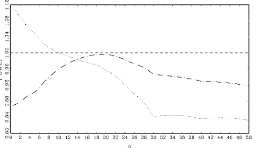
so that for all bandwidths, power was at least .999 for val-ues ofν above the truncation. Figure 1 plotsbopt for both the
Figure 1. Asymptotic Optimal Bandwiths for the Daniell Kernel ( Dan-J; Dan-BG).
JandBGscaling factors. In both cases,boptis relatively large
whenαis close to 0, andbopt declines asαincreases and the
errors become more stationary. The decline in bopt occurs in
somewhat discrete drops, likely due to the relative coarseness of the grid for α. Smoother functions for bopt could be
ob-tained with a finer grid at a substantially higher computational cost. Onceαis big enough,bopt drops to .02 and stays there.
Calculations done for the case of stationary errors confirm that
bopt=.02 for stationary errors. In the remainder of the article,
Dan-Jand Dan-BGdenote the Daniell kernel based tests, and they are always implemented using optimal bandwidths.
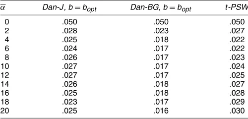
To show that Dan-Jand Dan-BGhave asymptotically correct size (due to the use of the scaling factors), Table 1 provides as-ymptotic null rejection probabilities of the Dan-Jand Dan-BG
statistics. Thet-PSW statistic is also included for comparison. Results are given forα=0,2,4, . . . ,18,20 at the 5% signif-icance level. In all cases rejection probabilities are no larger than .05, indicating that the scaling factors deliver tests that have asymptotically correct size.
Our power calculations reduce the number of potential tests in our class of tests from an infinite number to two. We are now in a position to address two interesting and practical questions: (1) How does the power of Dan-Jand Dan-BGcompare with each other and compare with power of t-PSW? and (2) How close is the power of Dan-J, Dan-BG, andt-PSWto the robust envelopes?
Figure 2 plots integrated power of the three tests relative to the integrated power of Dan-Jacross the grid forα. Obviously, the integrated power of Dan-Jrelative to itself is always 1. Two
Table 1. Asymptotic Null Rejection Probabilities in the Simple Trend Model Nearly Integrated Errors, 5% Nominal Level, 50,000 Replications
α Dan-J, b=bopt Dan-BG, b=bopt t-PSW
0 .050 .050 .050 2 .028 .023 .027 4 .025 .018 .022 6 .024 .017 .022 8 .026 .017 .023 10 .027 .017 .024 12 .027 .017 .025 14 .026 .018 .027 16 .025 .018 .028 18 .023 .017 .029 20 .025 .016 .030
Figure 2. Integrated Asymptotic Power Relative to Dan-J ( Dan-J; Dan-BG; t -PSW).
patterns stand out. First, notice that Dan-J dominates t-PSW
for all values ofα, although power is similar forα≈20. Sec-ond, the integrated power of Dan-Jand Dan-BGcross once at
α=10, and it is obvious that theBGscaling factor gives a more powerful test whenαis close to 0 and theJscaling factor gives a more powerful test for more stationary errors.
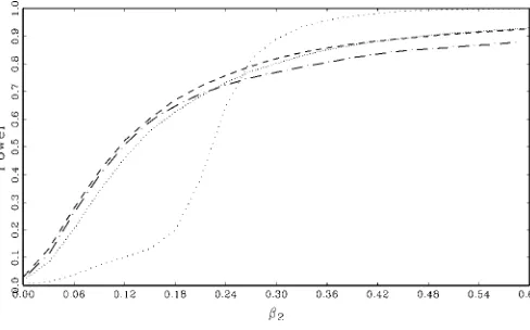
Figures 3–5 plot the asymptotic power (not the integrated power) of the tests along with the robust envelopes. Station-ary errors are depicted in Figure 3, and nearly integrated errors are depicted in Figures 4 and 5 with α=0,10. As an addi-tional benchmark, Figures 4 and 5 also include the power of a test based on infeasible generalized least squares (GLS). This power curve was easily computed analytically using theoretical results from Canjels and Watson (1997). In general, tests based on infeasible GLS dominate OLS-based tests forαclose to 0, whereas GLS and OLS are asymptotically equivalent for sta-tionary errors, as is known from the classic results of Grenander and Rosenblatt (1957). Figure 3 shows that in the case of sta-tionary errors, the Daniell kernel test usingbopt delivers a test
with power equal to the robust envelope, whereas the power oft-PSW lies below the robust envelope. Figure 4 shows that for α=0, the Dan-BGtest has power equal to the envelope. Dan-Jhas less power, although both Dan-BGand Dan-J dom-inatet-PSW. All of the OLS HAC tests are dominated by in-feasible GLS, as expected. Figure 5 shows that whenα=10, none of the tests attains the envelope. Dan-Jslightly dominates
Figure 3. Asymptotic Power Stationary Errors ( envelope; Daniell bopt; t -PSW).
Figure 4. Asymptotic Power I(1) Errors,α=0 ( infeasible GLS; robust-envelope; Dan-J bopt; Dan-BG bopt; t -PSW).
Dan-BG, and Dan-Jandt-PSWcross each other. These results are not surprising given the results in Figure 2.
The results given in Figures 2–5 should be interpreted with caution, because implementation of infeasible GLS, Dan-J, and Dan-BG requires a value of α that is an unknown parame-ter that cannot be consistently estimated. Canjels and Watson (1997) proposed a feasible version of GLS based on a simple proxy (i.e., inconsistent estimate) for α. These authors dealt with the uncertainty generated by using a proxy for α us-ing Bonferoni bounds. In subsequent sections we propose a straightforward data-dependent bandwidth rule that makes the Dan-J and Dan-BG tests feasible in practice, and we com-pare the finite-sample performance of the feasible tests with the
t-PSWstatistic.
7. A FEASIBLE DATA–DEPENDENT BANDWIDTH RULE
There are two challenges to implementing feasible versions of the Dan-J and Dan-BGtests. The first challenge is finding a simple function that can approximate the relationship between
bopt andα, as depicted in Figure 1. The second challenge is
dealing with the fact thatα is an unknown parameter that can-not be consistently estimated.
Let bopt(α) denote the function that gives optimal band-widths in terms of α. Given a value of α, it is easy (albeit
Figure 5. Asymptotic Power I(1) Errors,α=10 ( infeasible GLS; robust-envelope; Dan-J bopt; Dan-BG bopt; t -PSW).
computationally intensive) to computebopt(α). A practical
al-ternative is to approximatebopt(α)using the step-like functions
depicted in Figure 1. Let1(x≤a) denote the indicator function that takes on the value 1 ifx≤aand takes on the value 0 oth-erwise. The step function approximations forbopt(α), using the same simulations as for Figure 1, are as follows. For Dan-J,
bopt(α)=.02+.02·1(α≤21)+.02·1(α≤20)
+.04·1(α≤19)+.02·1(α≤18)+.12·1(α≤17) +.1·1(α≤14)+.1·1(α≤12)+.06·1(α≤11) +.12·1(α≤10)+.02·1(α≤7)+.2·1(α≤4), and for Dan-BG,
bopt(α)=.02+0.1·1(α≤29)+.02·1(α≤23)
+.02·1(α≤19)+.02·1(α≤17)+.02·1(α≤2). Based on the fact thatα=T(1−α), we can use these step functions to write the optimal bandwidth in terms of the sample size and an estimate ofα. The simplest estimator ofαis given by
α=
T
t=2utut−1
T t=2u2t−1
,
where theut’s are the OLS residuals from (7). Plugging into the formula forαgivesα=T(1−α), which can be used to define a data-dependent bandwidth rule given by
bopt=bopt
α. (9)
The bandwidth,M, used in the formula for (3) is given by
M=max(boptT,2), (10)
where the lower bound of 2 is placed onMto ensure thatMis not too small whenT andboptare both small.
We could follow Canjels and Watson (1997) and attempt to derive Bonferoni bounds when usingbopt. However, this
calcu-lation would be much more difficult than the calcucalcu-lations car-ried out by Canjels and Watson (1997). This is true because of the very complicated manner in whichαenters the asymp-totic distribution theory. In contrast, in the work of Canjels and Watson (1997),αentered the asymptotic distributions only through the variance of a normal random variable thus greatly simplifying the computation of Bonferoni bounds.
Although a theoretical analysis of the impact of usingbopt
on the asymptotic distributions of Dan-Jand Dan-BGis well
beyond the scope of this article, we can assess through finite sample simulations whether the following naive but simple as-ymptotic approximation works. Recall that the asas-ymptotic crit-ical value and the scaling factor,c, depend on the value ofb. A simple alternative to Bonferoni bounds is to use an asymp-totic critical value and a value forctreatingbopt as constant.
This approach is similar in spirit to the common practice of treating asymptotic variance estimators as known when us-ing standard first-order asymptotics. Althoughbopt is clearly
not constant (or even a consistent estimate of bopt)
finite-sample simulation results in the next section indicate that treat-ing it as consistent provides a remarkably accurate asymptotic approximation.
A final practical matter that merits discussion is finding a convenient way to obtain asymptotic critical values and the corresponding values ofcfor a given value ofbopt. Toward that
end, we took simulated asymptotic critical values and values ofcfor the grid ofb=.02, .04, . . . , .98,1.0 and estimated the following polynomial functions using OLS:
cv(b)=θ0+θ1b+θ2b2+θ3b3+θ4b4+θ5b5
and
c(b)=λ0+λ1b+λ2b2+λ3b3+λ4b4+λ5b5+λ6b6+λ7b7.
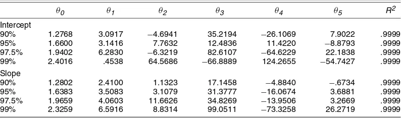
The estimated coefficients, along with theR2from the regres-sions, are given in Tables 2 and 3. In all cases, the fits are excel-lent. In practice, given a value ofboptand a significance level,
the value of cused for the scaling factor is given by c(bopt), and the rejection rule is carried out using the asymptotic crit-ical value given by cv(bopt). For convenience, we also report
cv(b)andc(b)functions for thet-statistic on the intercept para-meter in (7).
8. FINITE–SAMPLE EVIDENCE
In this section we discuss some finite-sample simulations designed to assess the accuracy of the asymptotic approxima-tions and to compare the finite-sample performance of the tests. We implemented the Dan-Jand Dan-BGtests using the feasible data-dependent bandwidth described in the previous section.
For the finite-sample simulations, we continue to use mo-del (7). We test the hypothesis that β2≤0 against β2>0 at the 5% significance level. The errors are generated accord-ing to ut =αut−1+et+φet−1, whereet is iid N(0,1). The first set of simulations assesses the accuracy of asymptotic
Table 2. Asymptotic Critical Value Function Coefficients of HAC Robust t -Tests in the Simple Linear Trend Model Using the Daniell Kernel, yt=β1+β2t+ut, cv(b)=θ0+θ1b+θ2b2+θ3b3+θ4b4+θ5b5
θ0 θ1 θ2 θ3 θ4 θ5 R2
Intercept
90% 1.2768 3.0917 −4.6941 35.2194 −26.1069 7.9022 .9999 95% 1.6600 3.1416 7.7632 12.4836 11.4220 −8.8793 .9999 97.5% 1.9402 6.2830 −6.3219 82.6107 −64.6229 22.1838 .9999 99% 2.4016 .4538 64.5686 −66.8889 124.2655 −54.7427 .9999 Slope
90% 1.2802 2.4100 1.1323 17.1458 −4.8840 −.6734 .9999 95% 1.6383 3.5083 3.1079 31.3777 −16.0674 3.6881 .9999 97.5% 1.9659 4.0603 11.6626 34.8269 −13.9506 3.2669 .9999 99% 2.3259 6.5916 8.8314 99.0511 −73.3258 26.2719 .9999
Table 3. Asymptotic c(b) Function Coefficients of HAC Robust t -Tests in the Simple Linear Trend Model Using the Daniell Kernel, yt=β1+β2t+ut, c(b)=λ0+λ1b+λ2b2+λ3b3+λ4b4+λ5b5+λ6b6+λ7b7
J scaling factor
λ0 λ1 λ2 λ3 λ4 λ5 λ6 λ7 R2
Intercept
90% .7499 −9.7621 65.796 −247.4533 528.4285 −634.3561 398.1199 −101.5139 .9970 95% .9610 −13.1521 90.3259 −343.243 736.7416 −886.1946 556.2731 −141.7148 .9965 97.5% 1.1890 −16.7142 115.2884 −438.3496 940.2971 −1,130.4387 709.5573 −180.8483 .9967 99% 1.5870 −24.2006 172.7681 −664.5252 1,429.5649 −1,717.8948 1,076.238 −273.5812 .9957 Slope
90% 1.1531 −10.7044 69.5348 −255.9725 540.5918 −644.6063 402.3978 −102.0847 .9974 95% 1.5765 −14.479 95.252 −356.2578 762.0497 −918.8257 579.6667 −148.584 .9970 97.5% 2.1582 −20.7712 142.0705 −541.8446 1,164.2989 −1,400.0856 878.4994 −223.8275 .9969 99% 2.9487 −27.6477 189.1506 −735.8488 1,615.5392 −1,979.9895 1,262.2460 −325.801 .9969
BG scaling factor
λ0 λ1 λ2 λ3 λ4 λ5 λ6 λ7 R2
Intercept
90% 234.2704 −2,868.4772 18,811.8039 −69,731.2231 147,463.4333 −175,665.7364 109,539.4716 −27,779.3683 .9981 95% 286.3570 −3,743.1267 25,162.8573 −94,152.1563 199,276.5117 −236,651.833 146,849.1402 −37,028.7816 .9980 97.5% 352.1194 −4,943.2405 34,469.1564 −131,258.8606 279,704.2615 −332,970.252 206,834.2458 −52,197.0985 .9980 99% 444.8561 −6,743.2306 48,990.1553 −190,438.6854 409,721.2544 −489,543.7975 304,130.5416 −76,587.1552 .9974 Slope
90% 354.9211 −3,192.5493 20,104.5508 −71,791.6215 149,125.4086 −176,601.0298 110,082.5451 −27,966.1682 .9970 95% 458.5817 −4,320.4082 28,274.2022 −101,854.4156 210,053.0637 −245,890.3349 151,589.8660 −38,163.0692 .9972 97.5% 577.7701 −5,475.1849 35,431.5583 −122,293.2595 238,753.4663 −264,497.7570 154,988.5891 −37,301.4541 .9978 99% 739.8640 −7,189.0036 48,398.4732 −172,687.4149 347,792.5436 −397,333.0643 239,910.1386 −59,396.9866 .9970
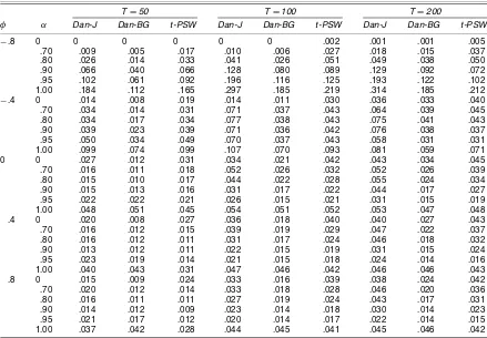
approximations under the null. Simulations are reported for
α=0, .7, .8, .9, .95,1.0;φ= −.8,−.4,−0, .4, .8; and sample sizes 50, 100, and 200. In all cases, 5,000 replications were
used. Table 4 provides empirical null rejection probabilities of the t-tests. It is clear that unless a large negative moving av-erage term and a unit root are simultaneously present, all of
Table 4. Empirical Null Rejection Probabilities in the Simple Trend Model 5% Nominal Level, 5,000 Replications, yt=β1+β2t+ut, ut=αut−1+et+φet−1, etIs iid N(0, 1), u0=0, H0:β2≤0, HA:β2>0
T=50 T=100 T=200
φ α Dan-J Dan-BG t-PSW Dan-J Dan-BG t-PSW Dan-J Dan-BG t-PSW
−.8 0 0 0 0 0 0 .002 .001 .001 .005
.70 .009 .005 .017 .010 .006 .027 .018 .015 .037 .80 .026 .014 .033 .041 .026 .051 .049 .038 .050 .90 .066 .040 .066 .128 .080 .089 .129 .092 .072 .95 .102 .061 .092 .196 .116 .125 .193 .122 .102 1.00 .184 .112 .165 .297 .185 .219 .314 .185 .212
−.4 0 .014 .008 .019 .014 .011 .030 .036 .033 .040
.70 .034 .014 .031 .071 .037 .043 .064 .039 .045 .80 .034 .017 .034 .077 .038 .043 .075 .041 .043 .90 .039 .023 .039 .071 .036 .042 .076 .038 .037 .95 .050 .034 .049 .070 .037 .043 .058 .031 .031 1.00 .099 .074 .099 .107 .070 .093 .081 .059 .071 0 0 .027 .012 .031 .034 .021 .042 .043 .034 .045 .70 .016 .011 .018 .052 .026 .032 .052 .026 .039 .80 .015 .010 .017 .044 .022 .028 .055 .024 .034 .90 .015 .013 .016 .031 .017 .022 .044 .017 .027 .95 .022 .022 .021 .026 .015 .021 .031 .015 .019 1.00 .048 .051 .045 .054 .051 .052 .053 .047 .048 .4 0 .020 .008 .027 .036 .018 .040 .040 .027 .043 .70 .016 .012 .015 .039 .019 .029 .047 .022 .037 .80 .016 .012 .011 .031 .017 .024 .046 .018 .032 .90 .013 .012 .011 .022 .015 .019 .031 .015 .024 .95 .023 .019 .014 .021 .015 .018 .024 .014 .016 1.00 .040 .043 .031 .047 .046 .042 .046 .046 .043 .8 0 .015 .009 .024 .033 .016 .039 .038 .024 .042 .70 .020 .012 .014 .033 .018 .028 .046 .020 .036 .80 .016 .011 .011 .027 .019 .024 .043 .017 .031 .90 .014 .012 .009 .023 .014 .018 .030 .014 .023 .95 .021 .017 .012 .020 .014 .017 .022 .014 .015 1.00 .037 .042 .028 .044 .045 .041 .045 .046 .042
NOTE: The feasible optimal bandwidth given by (10) was used for Dan-Jand Dan-BG.
Figure 6. Finite-Sample Power, AR(1) Errors, α=.7, T =100 ( Dan-J; Dan-BG; t -PSW; feasible GLS).
these tests have empirical rejection probabilities either close to or below .05. Therefore, theJandBGscaling factors work well in practice. This contrasts with standard HAC robust tests, for which it is well known that strong serial correlation causes overrejections that can be severe (see Vogelsang 1998, table I). The tests overreject when there is a unit root and a large nega-tive moving average component because theJandBGstatistics are oversized as unit root tests. In other words,JandBGtend to be too small in finite samples, and they do not scale down the
t-statistics sufficiently to control the overrejection problem. The overall performance of Dan-Jand Dan-BGin terms of size is similar tot-PSW and is quite impressive. These results suggest that treatingboptas constant is a reasonable approach.
We also report some finite-sample power results to show that in practice, power is qualitatively similar to that implied by the local asymptotic analysis. For comparison purposes, we also in-clude the power of a conservative feasible GLS test suggested by Canjels and Watson (1997). We implement this test in ex-actly the same manner as in the finite-sample power simula-tions reported by Vogelsang (1998). Figures 6–8 plot power for
α=.7, .9,1.0,φ=0, forT=100. The results show that the as-ymptotic patterns are also reflected in the finite-sample results. Dan-Jdominatest-PSWin all cases, whereas Dan-Jdominates Dan-BGexcept whenα=1. Perhaps as expected, whenα=1, the feasible GLS test has much higher power than the OLS-based tests. However, forα <1, feasible GLS can have much lower power than the OLS-based tests.
Figure 7. Finite-Sample Power, AR(1) Errors, α=.9, T =100 ( Dan-J; Dan-BG; t -PSW; feasible GLS).
Figure 8. Finite-Sample Power, AR(1) Errors, α=1.0, T =100 ( Dan-J; Dan-BG; t -PSW; feasible GLS).
Because of the well-known downward bias ofαin models with deterministic trends, we experimented using the median unbiased estimator ofαproposed by Andrews (1993) in place ofα when computingbopt. Although size results were
simi-lar, power was often lower using the median unbiased estimator of α. An interesting topic for future research will be to more carefully compare the relative merits of various methods of es-timatingαwhen constructingbopt.
Based on the results of this section, we recommend using the Dan-Jtest be used in practice. The power of Dan-J domi-natest-PSW, and Dan-Jhas much higher power than feasible GLS when α is not close to 1. We do not recommend using Dan-BGin practice, because in the one situation where Dan-BG
has higher power than Dan-J, feasible GLS has much higher power than both.
9. EVIDENCE ON THE PREBISCH–SINGER HYPOTHESIS
In this section we provide empirical evidence on the Pre-bisch–Singer hypothesis. The time series that we analyze is the logarithm of the net barter terms of trade series constructed by Grilli and Yang (1988) and extended by Lutz (1999) (see Grilli and Yang 1988; Lutz 1999 for details on the construction of this time series). The data are annual from 1900 to 1995. The net barter term of trade is the ratio of a nonfuel primary commodities price index to a manufacturing price index. The Prebisch–Singer hypothesis asserts that the net barter terms of trade should be falling over time. Figure 9 shows that the loga-rithm of net barter terms of trade has been decreasing over time. Is this decrease systematic? If we take regression (7) as a rea-sonable model of the statistical time series behavior of the loga-rithm of the net barter terms of trade, then the Prebisch–Singer hypothesis asserts that the trend slope coefficient is negative. If we take as the null hypothesis that the Prebisch–Singer hy-pothesis does not hold against the alternative that the Prebisch– Singer hypothesis holds, then we can parameterize the hypoth-esis asH0:β2≤0,H1:β2>0.
Note that the Prebisch–Singer hypothesis is an empirical no-tion about the long-run behavior of a time series; namely, that the time series is steadily decreasing over time. It is important to keep in mind that this notion has nothing to do with the correla-tion in the data. More specifically, the Prebisch–Singer hypoth-esis has nothing to do with whether the error term is stationary
Figure 9. Logarithm of Net Barter Terms of Trade and Fitted Trend.
or has a unit root. In our opinion, the empirical literature on the Prebisch–Singer hypothesis has become distracted by the unit root issue. This is not surprising given the technical difficulties the presence of a unit root brings with it. The advantage of the test proposed in this article is that it allows a direct and very simple test of the Prebisch–Singer hypothesis that does not de-pend on whether or not a unit root is in the errors.
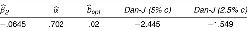
Using the logarithm of the net barter terms of trade series, we estimated regression (7) by OLS and obtained β2= −.0645.
We computed Dan-J, the recommended test, using the data-dependent bandwidth. Recall that the value of cused for the scaling factors depends on the significance level of the tests, and we provide results for significance levels 5% and 2.5%. The results, along withαandbopt, are reported in Table 5. The null
hypothesis that the Prebisch–Singer hypothesis does not hold can be rejected at the 5% level but not at the 2.5% level. This rejection is robust because the tests do not suffer from overre-jection problems even if the errors have a unit root. Our em-pirical result suggests that there is relatively strong evidence indicating that the Prebisch–Singer hypothesis holds, implying that Prebisch and Singer were right.
As an additional robustness check, we applied the partial sum trend function structural change tests proposed by Vogelsang (1999). We computed variants of the Vogelsang (1999) tests designed to jointly detect a shift in intercept and/or slope in the deterministic trend function. We treated the break date as unknown. The tests also use the J scaling factor to control the overrejection problem caused by strong serial correlation. We computed the mean, mean-exponential, and supremum sta-tistics using 1% trimming (see Vogelsang 1999 for details). The results were mean, .084; mean-exponential, .0103, and supremum, .0948. The 5% asymptotic critical values for these tests when using the J scaling factor were 2.0917, 1.3325, and 5.1651. Therefore, the null hypothesis that the trend func-tion is stable over time cannot be rejected.
Table 5. Empirical Results for the Logarithm of Net Barter Terms of Trade Annual Data, 1900–1995, Dan-J Statistic
β2 α bopt Dan-J (5% c) Dan-J (2.5% c)
−.0645 .702 .02 −2.445 −1.549
NOTE: The 5% and 2.5% asymptotic critical values are−1.710 and−2.052.
10. CONCLUSION
In this article we have proposed tests for hypotheses on the parameters of the deterministic trend function of a univariate time series. The tests do not require knowledge of the form of serial correlation in the data, and they are robust to strong serial correlation. Even when the data contain a unit root, the tests still have the correct size asymptotically. The tests that we analyzed are standard OLS HAC robust tests based on nonparametric variance estimators. We extended the fixed-basymptotic frame-work for HAC robust tests recently proposed by Kiefer and Vogelsang (2002), which allowed us to analyze the power prop-erties of the tests with regards to bandwidth and kernel choices. Our analysis showed that among popular kernels, the Daniell kernel delivers tests with optimal power within a specific class of tests that have the correct asymptotic size whether the er-rors are stationary or have a unit root. We achieved this size robustness using the J scaling factor proposed by Vogelsang (1998) and a new scaling factor, BG, based on the unit root test of Breitung (2002). Based on our asymptotic and finite-sample analysis, we recommend using the J correction over theBGcorrection in practice. Our results also suggest that the Dan-J test dominates the t-PSW test of Vogelsang (1998) in terms of power, and thus Dan-Jis recommended in practice.
We addressed the traditionally difficult issue of HAC band-width choice using fixed-basymptotics in conjunction with lo-cal to unity asymptotics. For a given value of the lolo-cal to unity parameter, we numerically determined the bandwidth that max-imizes integrated power. To our knowledge, this is the first bandwidth analysis focusing on the power of tests rather than on the mean squared error of the HAC estimate. Our analysis provides a data-dependent bandwidth that maximizes integrated power. Finite-sample simulations suggest that a feasible version of the optimal bandwidth rule works well in practice.
We applied the Dan-J test to the logarithm of a net barter terms of trade series; and the results suggest that this series has a statistically significant negative slope. This finding is consis-tent with the well-known Prebisch–Singer hypothesis. Because our tests are robust to strong serial correlation or a unit root in the data, our results in support of the Prebisch–Singer hypothe-sis are robust.
ACKNOWLEDGMENTS
The authors thank Alastair Hall, an associate editor, and two referees for thoughtful and constructive comments that lead to improvements of the article. They also thank Jan Jacobs for use-ful discussions, as well as seminar participants at the Univer-sity of Groningen, UniverUniver-sity of Tilburg, Iowa State UniverUniver-sity (Statistics), Cornell University, and the American Statistical Association Meetings (August 2000) for beneficial feedback. Vogelsang thanks the Center for Analytic Economics at Cornell and gratefully acknowledges support from National Science Foundation grant SES-0095211. The authors are grateful to Matthias Lutz, who kindly provided the data used in the article.
APPENDIX A: PROOF OF THEOREM 1
Here we give the proof of Theorem 1. Theorem 2 follows easily from Theorem 1 using simple algebra, and thus details are omitted.
A.1 Proof of Part (a)
Following Kiefer and Vogelsang (2002), we define
2κij=
and use this expression to rewriteσ2as
σ2= −T−1
For (A.1) to be valid, the residuals must sum to 0. So for the asymptotic results to hold, a constant must be included in the model. The following lemma provides the distribution ofT−1/2St.
Lemma A.1. T−1/2S[rT]⇒σQF(r).
Proof of Lemma A.1. Simple matrix manipulations yield
T−1/2S[rT]=T−1/2 Clearly, the terms consisting only of trend functions will have limiting distributions that do not depend on whether or notutis stationary. It is well known that these terms have the following limits:
The last term in (A.3) and the first term in (A.2) depend onut, and therefore their limiting distributions will depend on whether or not ut is stationary. Again using standard results, those asymptotic distributions are
Using these limits, the asymptotic distribution ofS[rT]is as fol-lows:
The rest of the proof is split into three cases, corresponding to type 1, type 2, and the Bartlett kernels.
Case 1. k(x)is a type 1 kernel. By definition of the second Vogelsang (2002), we use simple algebra and the definition of 2κij to establish that when|i−j|>[bT],2κij=0, and when|i−j| = [bT],2κij= −k([bT[bT]−]1). When|i−j|<[bT],
T22κij→k′′. First, consider the case when|α|<1. We split up the expression ofσ2as follows:
σ2 = T−1
= T−1
where the asymptotic distribution follows directly from Lemma A.1 and results of Kiefer and Vogelsang (2002). The result whenα=1−αT follows analogously forT−2σ2, where
Siis normalized byT−3/2instead ofT−1/2.
Case 3. k(x)is the Bartlett kernel. Here, again using simple algebra following Kiefer and Vogelsang (2002), it can be ver-ified that when|i−j| =0, 2κij=[bT2], when |i−j| = [bT],
2κij= −[bT1], and2kij=0 otherwise. Using these expres-sions and Lemma A.1 in (A.1), we obtain the following limiting distribution when|α|<1: paring the distributions from Cases 1–3 with the definition ofF(b,k)completes the proof of part (a).
A.2 Proof of Part (b)
First, note thatWT can be written as
WT =(Rβ−d)′ asymptotic distribution ofσ2 in part (a). Therefore, it follows directly that when|α|<1,
When α=1−αT, the desired result follows by normalizing
(β−β)byT−1/2and normalizingσ2 byT−2. Part (c) of the theorem follows directly from part (b).
APPENDIX B: LIST OF KERNELS
The kernels that we use are as follows:
Bartlett k(x)=
The second derivatives of the kernels we use are as follows:
Parzen (a) k′′(x)=
−12+36|x| for|x| ≤12 12(1− |x|) for 12≤ |x| ≤1;
QS k′′(x)=
Note that in the case of the Bartlett kernel, the asymptotic dis-tribution is not expressed in terms ofk′′(x), becausek′′(0)does not exist for the Bartlett kernel. The fact thatk′′(0)does not ex-ist does not pose any technical problems, because results for the Bartlett kernel are obtained through direct calculations.
[Received May 2003. Revised October 2004.]
REFERENCES
Andrews, D. W. K. (1993), “Exactly Median-Unbiased Estimation of First-Order Autoregressive/Unit Root Models,”Econometrica, 61, 139–165. Andrews, D. W. K., and Ploberger, W. (1994), “Optimal Tests When a
Nui-sance Parameter Is Present Only Under the Alternative,”Econometrica, 62, 1383–1414.
Ardeni, P. G., and Wright, B. (1992), “The Prebisch–Singer Hypothesis: A Reappraisal Independent of Stationarity Hypotheses,”Economic Journal, 102, 803–812.
Breitung, J. (2002), “Nonparametric Tests for Unit Roots and Cointegration,”
Journal of Econometrics, 108, 343–363.
Canjels, E., and Watson, M. W. (1997), “Estimating Deterministic Trends in the Presence of Serially Correlated Errors,”Review of Economics and Statistics, 79, 184–200.
Chan, N. H., and Wei, C. (1988), “Limiting Distribution of Least Squares Es-timates of Unstable Autoregressive Processes,”The Annals of Statistics, 16, 367–401.
Cuddington, J. T., and Urzua, C. M. (1989), “Trends and Cycles in the Net Barter Terms of Trade: A New Approach,”Economic Journal, 99, 426–442. Grenander, U., and Rosenblatt, M. (1957),Statistical Analysis of Stationary
Time Series, New York: Wiley.
Grilli, E. R., and Yang, C. (1988), “Primary Commodity Prices, Manufactured Goods Prices, and the Terms of Trade of Developing Countries,”World Bank Economic Review, 2, 1–47.
Hall, A. (2004),Generalized Method of Moments, Oxford, U.K.: Oxford Uni-versity Press.
Kiefer, N. M., and Vogelsang, T. J. (2002), “A New Asymptotic Theory for Heteroscedasticity-Autocorrelation Robust Tests,” working paper, Center for Analytic Economics, Cornell University.
Lutz, M. G. (1999), “A General Test of the Prebisch–Singer Hypothesis,”
Review of Development Economics, 3, 44–57.
Park, J. Y. (1990), “Testing for Unit Roots and Cointegration by Variable Addition,” inAdvances in Econometrics: Cointegration, Spurious Regres-sions and Unit Roots, eds. T. Fomby and F. Rhodes, London: Jai Press, pp. 107–134.
Park, J. Y., and Choi, I. (1988), “A New Approach to Testing for a Unit Root,” Working Paper 88-23, Center for Analytic Economics, Cornell University. Phillips, P. C. B. (1987), “Time Series Regression With Unit Roots,
Economet-rica, 55, 277–302.
Phillips, P. C. B., and Solo, V. (1992), “Asymptotics for Linear Processes,
The Annals of Statistics, 20, 971–1001.
Powell, A. (1991), “Commodity and Developing Country Terms of Trade: What Does the Long Run Show?”Economic Journal, 101, 1485–1496.
Prebisch, R. (1950), “The Economic Development of Latin America and Its Principle Problems, New York: United Nations Publications.
Sapsford, D. (1985), “The Statistical Debate on the Net Barter Terms of Trade Between Primary Commodities and Manufactures: A Comment and Some Additional Evidence,”Economic Journal, 95, 781–788.
Singer, H. (1950), “The Distributions of Gains Between Investing and Borrow-ing Countries,”American Economic Review, Papers and Proceedings, 40, 473–485.
Spraos, J. (1980), “The Statistical Debate on the Net Barter Terms of Trade Between Primary Commodities and Manufactures,”Economic Journal, 90, 107–128.
Trivedi, P. K. (1995), “Tests of Some Hypotheses About Time Series Behav-ior of Commodity Prices,” inAdvances in Econometrics and Quantitative Economics: A Volume in Honor of C. R. Rao, Oxford, U.K.: Blackwell, pp. 383–412.
Vogelsang, T. J. (1998), “Trend Function Hypothesis Testing in the Presence of Serial Correlation Parameters,”Econometrica, 65, 123–148.
(1999), “Testing for a Shift in Trend When Serial Correlation Is of Un-known Form,” Working Paper 97-11, Center for Analytic Economics, Cornell University.