I.
INTRODUCTION
I.1.
B
ACKGROUNDTelaga Warna is a shallow basin lake, situated at 25 km southeast of Bogor. This
lake contains freshwater supporting a rich ecosystem, promoting the lives of three primate
species of Java such as Hylobates moloch (owa jawa), Presbytis comata (surili), Trachypithecus auratus (lutung), and Macaca fascicularis (monyet ekor panjang) (Hernowo, 2006). Considering to its function, the national government established its
status as Nature Reserve in 1981 through Ministry of Forestry Regulation No.
481/Kpts/Um/6/1981.
The sustainability of this ecosystem and its function in the future are questionable by
looking the situation around Telaga Warna. The permeable and fertile soils, high rainfall,
reliable supply of good quality water, good climatic conditions, availability of cheap labor,
and easy access to Bogor city, are the causes of horticultural industry and settlement
booming around the lake. The population has increased tremendously around the lake,
resulting in a proliferation of unplanned settlements. The rapid development seems not to
be decelerated among many speculations on the complex relationships between
resources, resource users, and subsequent disputes. Because of that, its function as
water catchments area preserving hydrological function to the lower land is facing
uncertainty in the longer term. It becomes an interesting case for natural resource
management, specifically to answer the question how to preserve this ecosystem which
surrounded by a very dynamic landscape (BKSDA Jawa Barat, 2005) .
Sustainable land use is a complex problem which containing several issues in
different fields and then need to be solved by integrating the information from different
field studies. It requires not only the information come from relation of natural condition
and natural process such as land cover change and soil erosion, but also the information
from analysis of socio-economic condition of the catchments area. It aims to prevent even
a small part of land losing their function or degraded. Lack of information about the
condition of land is one of important problem to know why most of soil in mountainous
area is degraded (Tuan, 2004). To comprehend such issue, many aspects and levels
using information from history to present needs to be considered (Mannaerts 1993). One
of the major factors that affect sustainable land use is soil erosion.
The relationship between land cover and soil erosion is obvious. The change of
land cover tends to affect the quantity of soil erosion. Hence, the information of soil
Above rationale encourage the investigation of soil erosion through land cover
change assessment in relation to the land use development for conserving Telaga Warna
in the long term. Under some limitation, the result of this study is expected to facilitate the
design of land use especially its natural condition (land cover) which minimize soil erosion in “Telaga Warna” catchments area.
I.2.
O
BJECTIVESThe objectives of the research are as follows:
1)
To analyze the relation of soil erosion with land cover change in Telaga Warna Nature Reserve using USLE model by means of Remote Sensing and GeographicalInformation System.
II.
LITERATURE REVIEW
II.1.
FACTORS AND CAUSES OF LAND DEGRADATIONFactors of land degradation are the biophysical processes and attributes that
determine the kind of degradation processes. These include land quality as affected by its
intrinsic properties of climate, terrain/landscape, vegetation, and biodiversity, especially
soil biodiversity. Causes of land degradation are the agents that determine the rate of
degradation. These are biophysical, socioeconomic, and political forces that influence the
effectiveness of processes and factors of land degradation (Eswaran et al., 2001;
Zerabruk, 2003).
Basically soil erosion by water is an interaction of two items, the water and the soil.
However, there are subsidiary factors that can influence the interaction between the two
items (Zerabruk, 2003). Hence, the rate and magnitude of soil erosion by water is
dominantly controlled by the following factors:
A. Rainfall erosivity and runoff
Both rainfall and runoff factors must be considered in assessing a water erosion
problem. Erosivity is the capacity of rainfall to cause erosion. It is a function of rainfall
intensity, rainfall amount, erosive rain, rainfall duration, and kinetic energy of rain
(Shestha, 2002; Zerabruk, 2003). The soil lost due to rainfall is directly related to the
duration and intensity. As the intensity increases so does the diameter of each raindrop.
In addition, as the size of each raindrop increases, so does the amount of energy
transferred to the soil when it hits the soil surface. Thus, the more energy a particular
raindrop possesses, the greater erosive capability it has. Surface runoff occurs when rainfall exceeds a soil’s maximum saturation level and all surface depression storage is filled to capacity. The amount of runoff can be increased if infiltration is reduced due to
soil compaction (Zerabruk 2003).
B. Soil erodibility
Erodibility of a soil is its vulnerability or susceptibility to erosion. The factors which
affect erodibility of a soil fall into three broad groups namely physical features of soils,
such as aggregate stability, particle size distribution, base minerals, organic carbon
content, clay mineralogy, infiltration capaciity, pore size, pore stability and moisture
holding capacity of soil, topographic features and management of the land (Shestha,
organic matter and improved soil structure have a greater resistance to erosion. Sand,
sandy loam and loam-textured soils tend to be less erodible than silt, very fine sand and
certain clay textured soils. Tillage and cropping practices, which lower soil organic matter
levels, cause poor soil structure, and result compacted soils that contributed to increases
in the soil erodibility. Soil erodibility index can be derived from nomographs or determined
using different methodes such as the simple field test.
C. Slope gradient and length
Naturally, high gradient of slope, the greater the amount of soil loss from erosion
by water will be. Soil erosion by water also increases as the slope length increases due to
the greater accumulation of runoff. Slope gradient and length can be determined from
field estimation (using clinometers, compas and measuring tape), topographic maps, and
DTM (Shestha, 2002; Zerabruk, 2003).
D. Vegetation/crop cover
Soil erosion potential is increased if the soil has no or very little vegetative cover of
plants and/or crop residues. Plant and residue cover protects the soil from raindrop impact
and splash, tends to slow down the movement of a surface runoff and allows excess
surface water to infiltrate. The erosion-reducing effectiveness of a plant and/or residue
cover depends on the type, extent and quantity of cover.
E. Conservation measures
Certain conservation measures can reduce water erosion. Tillage and cropping
practices, as well as land management practices, directly affect the overall soil erosion
problem and solution on a farm.
II.2.
P
OTENTIALS
OILL
OSSE
STIMATIONB
ASED ON THEU
NIVERSALS
OILL
OSSE
QUATION(USLE)
The USLE is a simple multiplicative model to calculate potential soil loss. The USLE can
be written as:
A = R * K * LS * C * P with:
A –computed spatial average soil loss per unit of area, expressed in t/ha/a.
K – soil erodibility factor – the soil-loss rate per erosion index unit for a specified soil as measured on a standard plot, which is defined as a 22.1 m length of uniform 9 % slope in continuous clean-tilled fallow.
L – slope length factor – the ratio of soil loss from the field slope length to soil loss from a 22.1 m length under identical conditions.
S – slope steepness factor – the ratio of soil loss from the field slope gradient to soil loss from a 9 % slope under otherwise identical conditions.
C – cover-management factor – the ratio of soil loss from an area with specified cover and management to soil loss from an identical area in tilled continuous fallow.
P – support practice factor – the ratio of soil loss with a support practice like contouring, strip cropping, or terracing, to soil loss with straight-row farming up and down the slope.
II.3.
R
EMOTES
ENSINGT
ECHNIQUES TOL
ANDD
EGRADATIOND
ETECTIONRemote sensing provides a convenient source of information but the data collected
by these instruments do not directly correspond to the information we need (Hill et al.,
1995b; Torrion, 2002). Remote Sensing has high potential for critical land data collection
due to large area coverage, regular time interval, spatial and spectral resolution and which
facilitates detection of degraded areas (De Jong, 1994; Torrion, 2002). For degradation
mapping, features whether they are directly or indirectly visible on the ground should be
considered. For this reason, signs of degradation features should be well considered.
Degradation features that must be checked in the field include: 1) signs of degradation on
bare ground, 2) signs of degradation provided by vegetation and land use, and 3) signs of
degradation provided by the terrain morphology (Torrion, 2002).
Torrion (2002) arrived at two basic approaches dealing with change detection; 1) the
comparative analysis of independently produced classification for different dates, and 2)
the simultaneous analysis of multi-temporal data. Different change detection techniques
include univariate image differencing, vegetation index differencing, image regression,
image ratioing, principal component analysis, post classification comparison, direct
multi-date comparison, change vector analysis and background substraction. Various
researchers use multi-sensor data in monitoring salt affected soils, water-logged and
eroded soils, and desertification (Tripathy et al., 1996; Torrion, 2002). Though researchers
devised best techniques to serve their purpose, these techniques seem to yield different
III.
MATERIALS AND METHOD
III.1.
T
IME ANDL
OCATION OFS
TUDYThe study area is situated in the Puncak, Bogor District, about 25 km southeast from
Bogor (Figures 3.1). Its geographic position is between 106,99° – 107,01° E longitude and 6,68° - 6,70° S latitude. The altitude range of the study area is about 1250 - 2000
meters a.s.l.
Figure 3.1. Location map of the study area
III.2.
E
QUIPMENTTable 3.1. Equipment used
No. Item Utilization
1. PC Desktop Intel IV, RAM 1GB
MB
Desktop computer for processing the data
2. Tablet PC, RAM 1 GB Portable computer used for ground truthing
3. GPS (Garmin GPSMap 176C) Global Positioning System receiver used to
acquire earth-referenced coordinates
4. ERDAS Imagine 8.5 Software used for image data processing
5. ArcView 3.2 Software used as a main GIS Desktop
application for map viewer, spatial analysis, and map layouting
6. Spatial Analyst Tool An ArcView extension for grid-based data
analysis
7. Soil Water Assessment Tool
(SWAT)
An ArcView extension for delineating watershed and catchment area
8. MS Excel Office application used to analyze the
statistics of the data or results
III.3.
D
ATAThe data is classified into two types, i.e. digital satellite imagery and vector data.
Landsat TM and Landsat ETM+ are the satellite imagery used for land cover extraction
and further for land cover change analysis. IKONOS imagery is used to help the
identification of land cover types. The data used in this study is shown in the Table 3.2.
Table 3.2. Satellite data
No. Satellite Imagery Acquisition
1. Landsat TM Path: 122, Row: 65, year 1991, 1994, and 1997
2. Landsat ETM+ Path: 122, Row: 65, year 2001, 2004, and 2006
3. IKONOS 2002
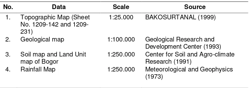
Digital vector data used are topographic and soil map. Contour feature from
topographic map was used to generate Digital Elevation Model (DEM) data. DEM,
geological and soil map is used in the analysis of soil erosion. The detail of the used
digital vector data are provided in the table below.
Table 3.3. Digital vector data
No. Data Scale Source
1. Topographic Map (Sheet
No. 142 and 1209-231)
1:25.000 BAKOSURTANAL (1999)
2. Geological map 1:100.000 Geological Research and
Development Center (1993)
3. Soil map and Land Unit
map of Bogor
1:250.000 Center for Soil and Agro-climate
Research (1991)
4. Rainfall Map 1:250.000 Meteorological and Geophysics
III.4.
M
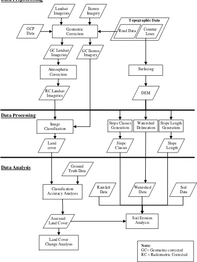
ETHODOLOGYDigital imagery data is the primary data of the study. These data must be prepared
before further analysis. Figure illustrates the overall process used for handling the data.
Figure 3.2. Overall image processing and analysis procedure
Note:
GC= Geometric corrected RC = Radiometric Corrected
Soil Data Classification
Accuracy Analysis
Soil Erosion Analysis Geometric
Correction
Atmospheric Correction
Surfacing Landsat
Imageries
Ikonos Imagery
Countur Lines Road Data
DEM GC Landsat
Imageries
GC Ikonos Imagery
Topographic Data
RC Landsat Imageries GCP
Data
Image Classification
Watershed Delineation
Ground Truth Data
Land Cover Change Analysis
Watershed Data Land
cover
Assessed Land Cover
Rainfall Data Data Processing
Data Analysis Data Preprocessing
Slope Classes
Slope Length Slope Classes
Generation
III.5.
D
ATA PREPROCESSINGThe aims of data preprocessing are to improve the quality of the images and to
produce the intermediate data which will be used in further processing. There are three
kind of data preprocessing done, i.e.: geometric correction, atmospheric correction, and
DEM generation. The description of the method of each process is given in the
subsections below.
A. Geometric Correction
Topographic map (especially road map) and Ground Control Point Data were used
as reference data to rectify IKONOS and Landsat data. Polynomial order was used for
developing transformation model and the used re-sampling method was cubic
convolution.
B. Atmospheric Correction
Atmospheric correction is conducted consider that the time when the satellite
captured the earth image, certain atmospheric condition occurred which affecting spectral
representation of features in image through the digital number. The atmospheric condition
may unique on each features but the reflectance value of features is always constant.
Therefore, to compare and process multi-date images data, the images should
radiometrically corrected in such that each feature has a similar reflectance value (digital
number) throughout the images.
In this research, relative radiometric normalization was used to improve the
radiometric quality of multi images efficiently. Another atmospheric correction method
used is haze removal. The description below describes the atmospheric correction used
in detail.
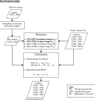
C. Relative Radiometric Normalization
Relative radiometric normalization (RRN) comprises of many methods, such as pseudo-invariant features, radiometric control set, image regression, no-change set
determined from scattergrams, and histogram matching (Yang and Lo, 2000). Image
regression (IR) based on pseudo-invariant features (PIF) is preferred consider that it is used to reduce variability throughout image other than land cover changes (Phua and
Tsuyuki, 2006) and possible to know the uncertainty level of developed model. It works
by using one image as reference and adjust the brightness of the rest image to match the
The dark object method was carried out upon Landsat images 2006 which is
assigned as referenced data of normalization. Even the image was suffered from striping
caused by Scan Line Corrector (SLC) failure, the radiometric quality remains intact
(USGS, 2006). The complete process of atmospheric correction can be seen in the figure
below.
Figure 3.3. The Process Flow of Atmospheric Correction
D. DEM Generation
DEM (Digital Elevation Model) is one of raster data used in this study which
generated from contour data. Contour data was came from topographic map (Rupa Bumi Indonesia map), sheet no. 1209-142 and 1209-231, with contour interval 12.5 m. DEM was generated through surfacing process by using non-linear rubber sheeting method. In
order to have same in resolution of data, DEM produced have a resolution as same as Atmospheric Correction:
dark object method Data Preprocessing
Landsat 12265_ 2006
Landsat 12265_ 1991 12265_ 1994 12265_ 1997 12265_ 2001 12265_ 2004 RC Landsat
12265_ 2006
PIS Selection
STD of PIS of reference image (σR(k))
STD of PIS of subject image (σS(k,y))
Mean of PIS of reference Image (Rk)
Mean of PIS of subject image (Sk,y )
Note:
PIS = Pseudo-invariant Set STD = Standard Deviation RC = Radiometric Corrected Transformation
Transformation Coefficient
slope: mk, y= σR(k) / σS(k,y)
intercept: bk, y = Rk - mk, y . Sk,y
Image Regression Model
Yy = mk, y . Xk + bk, y Reference Image
Subject Images (Xk)
Landsat 12265_ 1991 12265_ 1994 12265_ 1997 12265_ 2001 12265_ 2004
LANDSAT data, that is 30 m x 30 m. In further step of analysis in this study, the DEM was
converted to a slope map and then used as a one factor for estimate soil erosion.
III.6.
D
ATA PROCESSINGThere are three kinds of data processing are carried out to prepare the data for the
main analysis in the study (that is soil erosion analysis), comprise of image classification,
watershed delineation, and slope classes and length generation.
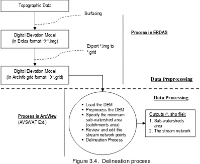
A. Watershed Delineation
The watershed delineation tool uses AVSWAT-2000 (version 1.0), the extension for ArcView and Spatial Analysis. It is used to perform watershed delineation based on
SWAT (Soil and Water Assessment Tool) model. SWAT is a model developed to predict the impact of land management practices on water, sediment, and agricultural chemical
yields in large, complex watershed with varying soils, land use, and management
conditions over long period of time (Arnold et al., 1998). The delineation process requires a Digital Elevation Model (DEM) in ArcInfo grid format. The diagram flow below illustrates
the steps in the delineation process:
Figure 3.4. Delineation process Topographic Data
Digital Elevation Model (in Erdas format *.img)
Digital Elevation Model (In ArcInfo grid format *.grid)
Surfacing
Export *.img to *.grid
Process in ERDAS
Outputs (*. shp file): 1.Sub-watersheds
area
2.The stream network Load the DEM
Preprocess the DEM Specify the minimum sub-watershed area (catchments area) Review and edit the
stream network points Delineation Process
Process in ArcView
(AVSWAT Ext.)
Figure 3.5 shows the catchments area which generated from Digital Elevation
Model (DEM). Delineating process obtained three large watersheds, which overlapped
with Telaga Warna Nature Reserve, as follows: Ciliwung, Cigundul and Cibeet
watersheds. However, the area study is limited on the catchments area (part of
watershed) that has an upper stream region on nature reserve area. Figure 3.5.b. shows
that area study has eight catchments that have upper stream region on nature reserve
area.
Figure 3.5. Delineating catchments area
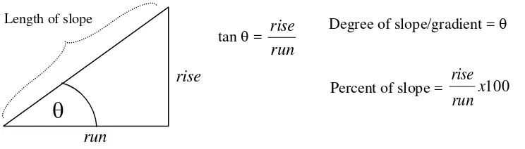
B. Slope Classes and Length Generation
The length and the gradient of the slope have a major influence on the amount of
soil erosion that can be occurred. The DEM was generated using surfacing method used
to produce length and gradient of the slope. The length and gradient of slope are
illustrated in the figure below:
The example of procedure: interval contour 25 m (rise) and distance 50 m (run), so length of slope is 55.9 m (Pythagoras Equation) and gradient of slope is 50 %.
tan =
run
rise
rise
run
Percent of slope =
x
100
run
rise
Length of slope Degree of slope/gradient =
n11 n12 n1k n1+
n21 n22 n2k n2+
nk1 nk2 nkk nk+
n+1 n+2 n+k n
Row total
Column total
Reference
C
lass
if
ic
at
ion
C. Classification Accuracy Analysis
Essentially, the procedure of accuracy assessment (Congalton and Green, 1999;
USGS, 2006b) can be summarized into two general procedures, i.e.: sampling design and
the assessment of accuracy parameters.
a. Sampling Design
Sampling definition
Sampling unit and size (total area in observation: 9629.23 ha, including watershed)
Sampling technique
b. Assessment of the Accuracy Parameters
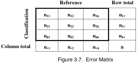
Figure 3.6. Possible Accuracy Categories of Classification
The accuracy parameters involve in building error matrix, estimating accuracy parameters such as total accuracy, user’s accuracy, and producer’s accuracy (Congalton and Green, 1999), KHAT statistic (Kappa estimator) and its variance. Error matrix describes the number of sample units (collected from reference data) assigned to three
possible accuracy categories, i.e.: correctly classified, misclassified and unclassified
categories (Figure 3.7.).
Figure 3.7. Error Matrix
is excluded from the category to which it belongs (Congalton and Green, 1999). The
design of error matrix is illustrated by Figure 3.7.
The following equations are used to calculate the accuracy parameters (Congalton
and Green, 1999):
Total (Overall) Accuracy (
P
ˆ
):n
n
P
k i ii
1ˆ
;
Producer’s Accuracy (
P
ˆ
A)
j jj j A n n P ˆ
User’s Accuracy (
PˆU):
i ii Uin
n
P
ˆ
Other accuracy parameter used is Kappa parameter, which estimated by computing
KHAT statistic. KHAT value is a measure of agreement (accuracy) based on the difference between actual agreement in the error matrix (the accuracy between
classification and reference data as indicated by the major diagonal) and the chance
agreement (as indicated by the row and column totals). In short, it is a measure how well
the classification agrees with reference data (Congalton and Green, 1999). The equation
of KHAT statistic is given below.
k i i i i k i i k i ii n n n n n n n K 1 2 1 1 ˆThe advantage of using KHAT statistic is that confidence interval around KHAT can
be computed. Additionally, it has normal distribution. Therefore, the hypothesis (whether
the significance of the agreement between the classification and there reference data is
greater than 0) can be formulated and tested. The equation used to compute variance of
KHAT statistic is shown in the following equations (Congalton and Green, 1999):
nii : diagonal elements of error matrix at i-th row and i-th column
i : the i-th row of error matrix
n : total number of sample units
j A
Pˆ : Producer’s accuracy at j-th class
njj : diagonal elements of error matrix at j-th row and j-th column
n+j : total number of sample units in j-th column
i U
Pˆ : Producer’s accuracy at i-th class
nii : diagonal elements of error matrix at i-th row and i-th column
4 2 2 2 4 2 1 3 2 3 2 1 1 2 2 1 11
4
1
1
2
1
2
1
1
1
)
ˆ
(
var
n
K
;
k i iin
n
1 11
;
k i i in
n
n
1 2 21
;
k i i i iin
n
n
n
1 2 31
;
k i k j i j ij n nn
n 1 1
2 3
4
1
The test statistic for testing the significance of KHAT statistic from a single error
matrix is expressed by:
)
ˆ
(
var
ˆ
1K
K
Z
The null hypothesis is rejected when Z ≥ Zα/2, where α/2 is the confidence level of
the two-tailed Z test.
D. Land Cover Change Analysis
The method used for analyzing land cover change per year was Boolean method.
Subsequently, the descriptive statistics in the tabular and graphic format was used to
expose the change of each class in sequential years. The analysis was carried out by
using MS Excel.
III.7.
S
OIL EROSION ANALYSISThe erosion is estimated by using USLE (Universal Soil Loss Equation) model (Wischmeier dan Smith, 1978). The model is ordered several factors which presumed
affected land erosion, which mathematically describe by the equation below:
A = R x K x LS x C x P
A : Maximum soil erosion rate (ton/ha/year) R : Rain erosivity factor
K : Soil erodibility factor
C : Plant management factor index
P : Soil conservation techniques factor index
1. Erosivity Factor
Erosivity factor is estimated by considering monthly rainfall intensity (r), rainy days (D), and maximum rainfall intensity (M) in 24 hours. The equation is given below (Bols, 1978):
EI
30= 6,119 .r
1,21.D
-0,47. M
0,532. Erodibility Factor
Soil erodibility is estimated based on soil sensitivity on erosion, which influenced by
the nature of soil texture, structure, permeability and contained bio-organic matters.
100 K = 1.292 [2.1 M
1.14(10
-4) (12-a)] + 3.25 (b-2) + 2.5 (c-3)
where:
M : (% sand + % dust) x (100 - % clay) a : soil organic matter concentration (%) b : soil structure codes
c : soil permeability classes
3. Slope and length factor
The length slope (LS) is estimated by the following equation below (Ardis and Booth, 2004):
NNconst length slope
slope slope
LS
0.065 0.0456. 0.00654. 2 _
Where:
slope : slope steepness (%) slope_length : length of slope (meter) const : a constant, i.e.: 22.1
NN : constant determined from Table Error! Reference
source not found..
Table 3.4. Slope Range and NN Exponent Constants (Arsyad, 1989)
No. Slope NN
1 < 1% 0.2
2 1% < slope < 3% 0.3
4. C and P Factor
C and P factor is determined by referring to the investigation of Arsyad (1989) and Wischmeier and Smith (1979 in Arsyad, 1989) and the information obtained from ground check data and image interpretation.
The relationship between land cover change and erosion rate was described by
projecting area of each land cover class and erosion rate into time line. The cumulative
IV.
RESULTS AND DISCUSSION
IV.1.
T
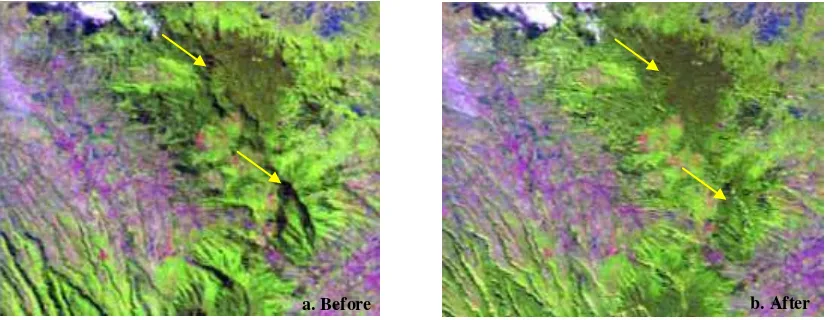
OPOGRAPHIC NORMALIZATION OF LANDSAT IMAGEThe area study is a mountainous area which certain parts have a significant
variation of topography. In turn, it affects the result of classification. Therefore,
topographic correction has to be done, before conducting classification. Topographic
slope, aspect, calculated incidence, and angle existence were merged with the
multi-spectral Landsat response for TM/ETM bands. In order to fit a generalized photometric
function, Minnaert method, a member of non-Lambertian model in which utilizing
regression analysis, was applied (Smith et al., 1980; Riano et al., 2003; Kato, 2003). Figures below show the results of the topographic normalization process.
Figure 4.1. Results of topographic normalization LANDSAT Image
Generally, the effect of topography was reduced. Previously, at the area which
has a high slope and aspect in line with solar radiation is darker than others, even they
has a same land cover type (Figure 4.1). Minnaert method was able to correct such error,
although it was overestimated for a small area which slopes more than 50 (Figure 4.1).
IV.2.
L
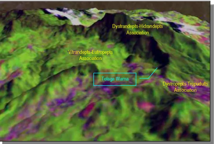
ANDSCAPE AND SOIL CLASSIFICATIONBased on Landsystem Map (Landsystem with Suitability and Environmental
Hazard, 1989), there are three soil associations found on the site location. They have
Figure 4.2. Landscape and soil classification
Soils of the Dystrandepts-Hydrandepts association occur in largely inaccessible
deep V-shaped drainages and narrow ridges on very steep west/east-facing slopes above
an elevation of about 1,500 meter a.s.l (above sea level), and serve primarily as a
watershed (Foote et al. 1972) (Figure 4.3.). These are thin, well-drained, light soils derived
from volcanic ash that are high in organic matter, can contain more water than other soil
when saturated, and are strongly to extremely acid. Because of their characteristics,
medium textured soils, such as the silt loam soils, this association have moderate K
values, about 0.25 – 0.40. They are moderately susceptible to detachment and produce
moderate runoff (http://www.iwr.msu.edu). Their occurrence on steep slopes, potential
friability at the surface, and fine silty texture, the soil erosion hazard by water is high for
this association, especially in areas where vegetation has been depleted. However, in
case a forest as cover vegetation, organic matter in their structure can reduces erodibility
because it reduces the susceptibility of the soil to detachment, and it increases infiltration
(Armas, 2004).
Association Dystrandepts-Hydrandepts
(Landsystem Type: TGM) Association
Vitrandepts-Eutropepts (Landsystem Type: CGS)
Association Dystropepts-Tropudults (Landsystem Type: BSM)
Ciliwung Hulu Cibeet
Figure 4.3. Description for soil type in study area
Vitrandepts-Eutropepts association is a porous soil, which developed from volcanic
ash (Hart et al, 2004). Depending on the above parent material and weathering force,
those soil type characterized by low soil organic matter, even though they is developed by
deposits material from upper area and leaching process not as intensive as upper area.
So have low K value, about 0.05 – 0.10, because erodibility can reduced if soil structure in stable caused by organic matter bounding.
Dystropepts-Tropudults association is a mature soil type, which weather process
intensively and high in clay.
IV.3.
L
AND COVER CHANGESBased on Landsat data there are 10 classes of land cover can be identified, which
are forest, bush/scrub, mix garden, built up, paddy field, upland, tea plantation, bare land,
grass and water.
In total 9629.23 ha of study area were evaluated for land cover changes. Table 4.1
presents about land cover changes from 1991 until 2006. In detail, land cover change Dystrandepts-Hidrandepts
Association
Vitrandepts-Eutropepts Association
Dystropepts-Tropudults Association
Table 4.1. a. Land cover changes from 1991 until 2006
1991 1994 1997 2001 2004 2006
(hectare)
Forest 3315.51 3162.60 2978.64 2726.73 2474.19 2000.340
Bush 1043.46 1027.62 1286.10 1171.62 1677.87 1393.660
Mix garden 574.74 898.47 422.64 804.78 409.06 824.490
Built up 133.11 255.06 352.35 457.65 743.76 1058.580
Paddy field 30.24 38.88 29.70 137.61 126.36 60.750
Upland 1172.25 904.32 1373.22 1215.99 977.13 920.250
Tea plantation 562.41 968.31 749.79 663.75 923.61 748.290
Bare land 763.83 318.42 301.68 124.29 224.56 582.22
Grass 8.46 29.88 111.24 310.77 53.01 21.24
Water 0.54 0.90 11.25 2.43 1.53 1.26
Cloud 4.14 4.14 4.14 4.14 4.14 4.14
Shadow 8.01 8.01 8.01 8.01 8.01 8.01
b. Trend cover changes from 1991 until 2006
1990-1994 1994-1997 1997-2001 1997-2004 2004-2006 Total Change (percent)
Forest -1.59 -1.91 -2.62 -2.62 -4.92 -13.69
Bush -0.16 2.69 -1.19 5.26 -2.95 3.64
Mixgarden 3.37 -4.95 3.97 -4.11 4.32 2.60
Builtup 1.27 1.01 1.09 2.97 3.27 9.63
Paddy field 0.09 -0.10 1.12 -0.12 -0.68 0.32
Upland -2.79 4.88 -1.63 -2.48 -0.59 -2.62
Tea plantation 4.22 -2.27 -0.89 2.70 -1.82 1.93
Bareland -4.64 -0.17 -1.84 1.04 3.72 -1.89
Grass 0.22 0.85 2.07 -2.68 -0.33 0.13
Water 0.00 0.11 -0.09 -0.01 0.00 0.01
Cloud 0.00 0.00 0.00 0.00 0.00 0.00
Shadow 0.00 0.00 0.00 0.00 0.00 0.00
The rates of land conversion between 1991, 1994, 1997, 2001, 2004 and 2006 are
given in Figure 4.4. The negative bars represent land types that decreased in extent,
F o re st Bu sh M ix g a rd e n Bu il tu p Pa d d y fi e ld U p la n d T e a p la n ta ti o n Ba re la n d G ra ss W a te r C lo u d Sh a d o w -6.00 -5.00 -4.00 -3.00 -2.00 -1.00 0.00 1.00 2.00 3.00 4.00 5.00 1990-1994 % C h a n g e Forest Bush Mixgarden Builtup Paddy field Upland Tea plantation Bareland Grass Water Cloud Shadow F o re s t B u s h M ix g a rd e n B u ilt u p P a d d y f ie ld U p la n d T e a p la n ta tio n B a re la n d G ra s s W a te r C lo u d S h a d o w -6.00 -4.00 -2.00 0.00 2.00 4.00 6.00 1994-1997 % C h a n g e Forest Bush Mixgarden Builtup Paddy field Upland Tea plantation Bareland Grass Water Cloud Shadow Fo re s t B u s h M ix g a rd e n B u ilt u p P a d d y f ie ld U p la n d T e a p la n ta ti o n Ba re la n d G ra ss W a te r C lo u d Sh a d o w -3.00 -2.00 -1.00 0.00 1.00 2.00 3.00 4.00 5.00 1997-2001 % C h a n g e Forest Bush Mixgarden Builtup Paddy field Upland Tea plantation Bareland Grass Water Cloud Shadow F o re st B u sh Mi xg a rd e n B u ilt u p P a d d y fi e ld U p la n d Te a p la n ta ti o n B a re la n d G ra s s W a te r C lo u d S h a d o w -6.00 -4.00 -2.00 0.00 2.00 4.00 6.00 1997-2004 % C h a n g e Forest Bush Mixgarden Builtup Paddy field Upland Tea plantation Bareland Grass Water Cloud Shadow F o re st B u sh M ix g a rd e n B u ilt u p P a d d y fi e ld U p la n d T e a p la n ta ti o n B a re la n d G ra ss W a te r C lo u d S h a d o w -6.00 -4.00 -2.00 0.00 2.00 4.00 6.00 2004-2006 % C h a n g e Forest Bush Mixgarden Builtup Paddy field Upland Tea plantation Bareland Grass Water Cloud Shadow
Figure 4.4. The rates of land cover conversion from 1991 until 2006
Based on result of classification, forest, bush, upland and bare land has decreased
between 1991 and 1994. However, upland and bare land fluctuate in next year. Its
fluctuating happened depends on a season and planting time. Decreasing forest cover
0.00 500.00 1000.00 1500.00 2000.00 2500.00 3000.00 3500.00
1991 1994 1997 2001 2004 2006
Year A re a ( he c ta re ) Forest Bush Mixgarden Builtup Paddy field Upland Tea plantation Bareland Grass Water Cloud Shadow 0.0 500.0 1000.0 1500.0 2000.0 2500.0 3000.0 3500.0
1991 1994 1997 2001 2004 2006
A re a ( he c ta re ) 0.0 200.0 400.0 600.0 800.0 1000.0 1200.0 Year A re a ( he c ta re ) Forest Builtup 0.0 200.0 400.0 600.0 800.0 1000.0 1200.0 1400.0 1600.0 1800.0
1991 1994 1997 2001 2004 2006
A re a ( he c ta re ) 0.0 100.0 200.0 300.0 400.0 500.0 600.0 700.0 800.0 900.0 Year A re a ( he c ta re )
Bush Mixgarden Paddy field Upland Tea plantation Bareland Grass Water Cloud Shadow
Figure 4.5. Land conversion processes from 1991 until 2006
Figure 4.5. shows land conversion processes between 1991 and 2006 with all
lands grouped in three clusters. Degradation of ecologically valuable land caused by
forest cover decreasing between 1991 until 2006 affects more than 13.66 % of the total
land area (over 1.315 ha). Moreover, 9.61 % of the built up/settlement (over 925 ha) and
9.48 % of cultivated land always in fluctuated depends on a seasons and planting time
(over 912 ha).
Between 1991 until 2006, bush, mix garden, built up, paddy field, tea plantation,
and grass increased per year by 0.24 %, 0.17 %, 0.64 %, 0.02 %, 0.13 % and 0.01 %,
respectively. Forest cover decreased by 1,315 ha representing decrease of 0.91 % per
1
2
year. Areas of upland and bare land also decreased between 1991 until 2006 by 0.17 %
and 0.13 % per year, respectively.
Upper Ciliwung
Cibeet
Cigundul
Telaga Warna Nature Reserve
Telaga Warna Lake
Upper Ciliwung
Cibeet
Cigundul
Telaga Warna Nature Reserve
Telaga Warna Lake
Upper Ciliwung
Cibeet
Cigundul
Telaga Warna Nature Reserve
Telaga Warna Lake
2006
Upper Ciliwung
Cibeet
Cigundul
Telaga Warna Nature Reserve
Telaga Warna Lake
2004
1991 1994
1997 2001
2004 2006
Upper Ciliwung
Cibeet
Cigundul
Telaga Warna Nature Reserve
Telaga Warna Lake
Upper Ciliwung
Cibeet
Cigundul
Telaga Warna Nature Reserve
0.00 100.00 200.00 300.00 400.00 500.00 600.00 700.00 800.00 900.00 1000.00
1991 1994 1997 2001 2004 2006
Year
A
re
a
(
he
c
ta
re
)
0.00 20.00 40.00 60.00 80.00 100.00 120.00 140.00 160.00 180.00
A
re
a
(
he
c
ta
re
)
Figure 4.6. Distributions of Land cover from 1991 until 2006
Figure 4.5. and 4.6. suggests that ecological causes behind almost 25 % (forest
and built up cover conversion) of the total area. At the same time, although in fluctuating
rate, but cultivated lands for agricultural productions tend to increase. These results
suggest that prospects for land preservation of upper Ciliwung, Cigundul and Cibeet
catchments area not very good without changes in policy. However, land preservation of
area Telaga Warna Nature Reserve is currently good.
Figure 4.7. shows that catchments area in upper Ciliwung, Cigundul and Cibeet
has different trend of forest and built up/settlement cover changes. Forest cover of upper
Ciliwung watershed has curve decrease stepper than Cigundul and Cibeet watershed.
During 5 years, built up cover in upper Cigundul watershed increased significantly.
Figure 4.7. Trend of forest and built up cover change in three catchments area
Increase of degraded land as product of land cover change during 1991–2006 will
be analyzed hereafter-using soil erosion approach.
IV.4.
A
CCURACY ASSESSMENT OF IMAGE CLASSIFICATIONIn this study, image data used are Landsat 1991 to 2006 and classified to 10
classes of land cover, but for accuracy assessment only conducted on image 2006,
because have limitation for ground control reference in the past.
The general acceptance of the error matrix as the standard descriptive reporting
tool for accuracy assessment of remotely sensed data has significantly improved the use
of such data. An error matrix is a square array of numbers organized in rows and columns
which express the number of sample units (i.e. pixels and clusters of pixels) assigned to a
particular category relative to the actual category as indicated by reference data
(Congalton, 1996).
An initial error matrix was generated for the initial supervised 2006 land cover map
prior to the mode filtering by creating a maximum likelihood report (Tabel 4.2). This report
calculates area and percentages of each land class incorporated in a maximum likelihood
classification. The ground truth data were utilized in the maximum likelihood report as the
independent data set from which the classification accuracy was compared. The
accuracy is essentially a measure of how many ground truth pixels were classified
correctly.
Table 4.2. Classification Accuracy Assessment Report
Error Matrix Accuracy
No Classified Data Ground truth
Forest Bush Mix garden Built up Paddy field Upland Tea planta Bare land Grass Water (Percent)
1 Forest 25 88.00 8.00 0.00 0.00 0.00 0.00 4.00 0.00 0.00 0.00
2 Bush 7 14.29 85.71 0.00 0.00 0.00 0.00 0.00 0.00 0.00 0.00
3 Mix garden 20 0.00 0.00 90.00 0.00 0.00 5.00 5.00 0.00 0.00 0.00
4 Built up 25 0.00 0.00 4.00 88.00 4.00 4.00 0.00 0.00 0.00 0.00
5 Paddy field 0 0.00 0.00 0.00 0.00 0.00 0.00 0.00 0.00 0.00 0.00
6 Upland 13 0.00 0.00 0.00 0.00 0.00 100.00 0.00 0.00 0.00 0.00
7 Tea plantation 21 0.00 4.76 0.00 0.00 0.00 0.00 95.24 0.00 0.00 0.00
8 Bare land 4 25.00 0.00 0.00 0.00 0.00 0.00 75.00 0.00 0.00 0.00
9 Grass 0 0.00 0.00 0.00 0.00 0.00 0.00 0.00 0.00 0.00 0.00
10 Water 0 0.00 0.00 0.00 0.00 0.00 0.00 0.00 0.00 0.00 0.00
Column Total 115 24 9 19 22 1 15 25 0 0 0
Accuracy Result
Class Names Reference Totals
Classified Totals
Number Correct
Producers
Accuracy Users Accuracy
Kappa Accuracy
1. Forest 24 25 22 91.67% 88.00% 0.85
2. Bush 9 7 6 66.67% 85.71% 0.85
3. Mix garden 19 20 18 94.74% 90.00% 0.88
4. Built up 22 25 22 100.00% 88.00% 0.85
Class Names Reference Totals
Classified Totals
Number Correct
Producers
Accuracy Users Accuracy
Kappa Accuracy
8. Bare land 0 4 0 --- --- 0.00
9. Grass 0 0 0 --- --- 0.00
10. water 0 0 0 --- --- 0.00
Totals 115 115 101
Overall Classification Accuracy = 87.83% Kappa Coefficient = 0.8525
An overall accuracy of 87.83% was achieved with a Kappa coefficient of 0.8525.
The overall accuracy is a similar average with the accuracy of each class weighted by the
proportion of test samples for that class in the total training of testing sets. Thus, the
overall accuracy is a more accurate of accuracy.
The importance and power of the Kappa analysis is that it is possible to test if a
land cover map is significantly better than if the map had been generated by randomly
assigning labels to areas (Congalton, 1996). It is widely used because all elements in the
classification error matrix, and not just the main diagonal, contribute to its calculation and
because it compensates for change agreement (Rosenfield & Fitzpatrick-Lins, 1986). The
Kappa coefficient represents the proportion of agreement obtained after removing the
proportion of agreement that could be expected to occur by chance (Foody, 1992).
This implies that the Kappa value of 0.8525 represents a probable 85% better accuracy
than if the classification resulted from a random, unsupervised, assignment instead of the
employed maximum likelihood classification.
The Kappa coefficient lies typically on a scale between 0 and 1, where the latter
indicates complete agreement, and is often multiplied by 100 to give a percentage
measure of classification accuracy. Kappa values are also characterized into 3 groupings:
a value greater than 0.80 (80%) represents strong agreement, a value between 0.40 and
0.80 (40 to 80%) represents moderate agreement, and a value below 0.40 (40%)
represents poor agreement (Congalton, 1996).
IV.5.
T
REND OF SOIL EROSIONIn this study, soil erosion in the whole watershed was estimated with GIS Remote
Sensing based on USLE. The rainfall factor R was assumed a constant value in the
whole study area, because study area not too wide, and no enough rainfall data available,
which accurate to determined rainfall map in detail scale. So, soil erosion rate in this
The result of calculation of soil erosion (soil loss risk) between 1991, 1994, 1997,
2001, 2004 and 2006 are given in Table 4.3 and Figure 4.8.
Table 4.3. Calculation of soil erosion from 1991 until 2006
No Class of
soil erosion
1991 1994 1997 2001 2004 2006
Area (hectare)
1 Very low 4921.47 5082.48 4814.82 4721.67 4467.78 3914.19
2 Low 1235.97 1267.38 1251.81 1257.57 1282.77 1366.65
3 Moderate 1278.90 1194.21 1416.24 1481.31 1721.61 1965.78
4 Heavy 149.13 100.17 149.13 164.52 147.24 259.11
5 Very heavy 111.78 53.01 65.25 72.18 77.85 191.52
1991 1994
Figure 4.8. Distribution of soil erosion rate from 1991 until 2006
In figure above, shows the effect of land cover change to soil erosion that analyzed
spatially and timely from 1991 until 2006. However, in figure above can seen that difficult
to make some trend of soil erosion rate from each years, because interact with land cover
factor change, and it is depend on season and planting time.
2004 2006
Figure 4.9. Cover change and very heavy class of soil erosion
Figure 4.9. shows the result of analysis about effect of land cover change to soil
erosion in pattern. Most areas with soil erosion rate in very heavy class happened if land
cover change to bare land, up land, mix garden and built up, although that location not in
steep of slope (more than 40 %). Very heavy class of soil erosion happened in bare land,
mix garden, up land, built up and grass. The area for that class in each year showed in
[image:30.595.82.531.653.763.2]table below.
Table 4.4. Relation landcover change and very heavy class of soil erosion
No Type of land cover 91-94 94-97 97-2001 2001-2004 2004-2006
Area (hectare)
1 Mix garden 2.07 1.44 6.66 0.99 5.22
2 Built up 0.72 1.71 5.22 10.98 28.53
3 Upland 3.96 20.70 24.21 13.32 21.60
4 Bare land 27.99 26.19 14.58 19.44 96.21
2004 2006
V.
CONCLUSION
Based on result of classification, decreasing forest cover happened consistently
until 2006, opposite with increasing in built up (settlement) cover. Cultivated area always
in fluctuated depends on a seasons and planting time. However, land preservation of area
Telaga Warna Nature Reserve is currently good.
The result of analysis about effect of land cover changes to soil erosion in pattern
has showed that most areas with soil erosion rate in very heavy class happened if land
cover change to bare land, up land, mix garden and built up, although that location not in
steep of slope (more than 40 %). Very heavy class of soil erosion happened in bare land,
mix garden, up land, built up and grass. The area for that class in each year showed in