IMPROVING ACTIVE QUERIES WITH A LOCAL SEGMENTATION STEP AND
APPLICATION TO LAND COVER CLASSIFICATION
S. Wuttkea,b,∗, W. Middelmanna, U. Stillab
a
Fraunhofer IOSB, Gutleuthausstr. 1, 76275 Ettlingen, Germany - (sebastian.wuttke, wolfgang.middelmann)@iosb.fraunhofer.de b
Technische Universitaet Muenchen, Arcisstr. 21, 80333 Muenchen, Germany - [email protected]
KEY WORDS:Active Learning, Remote Sensing, Land Cover Classification, Segmentation, Hierarchical Clustering, Active Queries
ABSTRACT:
Active queries is an active learning method used for classification of remote sensing images. It consists of three steps: hierarchical clustering, dendrogram division, and active label selection. The goal of active learning is to reduce the needed amount of labeled data while preserving classification accuracy. We propose to apply local segmentation as a new step preceding the hierarchical clustering. We are using the SLIC (simple linear iterative clustering) algorithm for dedicated image segmentation. This incorporates spatial knowledge which leads to an increased learning rate and reduces classification error. The proposed method is applied to six different areas of the Vaihingen dataset.
1. INTRODUCTION
Land cover is defined by the United Nations as “the observed (bio)physical cover on the earth’s surface” (Di Gregorio and Jan-sen, 2000). To make informed political, economic, and social de-cisions it is important to know which land cover type is found in different areas of the earth (Anderson, 1976). Climate studies for example are in need of precise information about the distribution of different land cover types. In urban planning it is important to differentiate between closed and open soil to predict the effects of rainfall.
Today’s constantly advancing remote sensing technology allows for higher resolutions, faster repetitions, and cheaper and there-fore more ubiquitous sensors. The availability of smaller form factors enables the development of multi sensor platforms (Harak´e et al., 2016). This leads to a manifold increase in available raw data. Processing these manually in a timely manner is impossible. To handle this challenge, advances in machine learning are neces-sary. To support this automation, two distinct information sources can be identified in remotely sensed data: spatial and spectral. The first is governed by the Smoothness Assumption (Schindler, 2012) which states that pixels have a higher probability of be-longing to the same class if they are spatially closer. The second information source is governed by the Cluster Assumption (Patra and Bruzzone, 2011) which states that pixels have a higher prob-ability of belonging to the same class if they are spectrally closer. These information sources are calledredundancies by (Hasan-zadeh and Kasaei, 2010). To exploit these information sources, unsupervised machine learning uses different segmentation and clustering techniques. This has the advantage that all available data can be used at once. The biggest disadvantage is that unsu-pervised techniques are hard to calibrate because of the missing explicit link between the unsupervised detected clusters and the classes of interest to the user (Fleming et al., 1975, Munoz-Mari et al., 2012, Lee and Crawford, 2004, Lee, 2004). In contrast, the supervised approach lets the user label instances with the desired class. This leads to improved classification results, but entails the additional costs of acquiring ground truth data. To gather these
∗Corresponding author
in a remote sensing setting often requires expensive ground sur-veys or the use of experts in image interpretation. Reducing these costs by strategically choosing which label to acquire is goal of the active learning approach (Atlas et al., 1990, Settles, 2012). Active learning is investigated thoroughly on a theoretical level (Balcan et al., 2006, Hanneke, 2014, K¨a¨ari¨ainen, 2006) as well as applied in a variety of fields such as bio-medical (Cui et al., 2009, Pasolli and Melgani, 2010, Krempl et al., 2015) and im-age retrieval (Cheng and Wang, 2007, Liu et al., 2008, Zhang et al., 2008). A good overview of applied active learning in re-mote sensing is given in (Tuia et al., 2011, Bruzzone and Persello, 2010). Applications particular for land cover classifications can be found in (Demir et al., 2012). To combine these available tools in a manner that is computationally efficient, conserving human interaction time, and achieving high classification results, is a challenging task.
The principle of using a hierarchy to guide the sampling follows the work of (Dasgupta and Hsu, 2008). They start with a tree hierarchy and try to find the optimal pruning which corresponds to the optimal segmentation. It is applied to remote sensing in (Tuia et al., 2012) as the active queries method. They introduce strategies to select the optimal node for splitting and to choose the optimal leaf for querying the user. The result is a three stage approach: 1) create a hierarchical clustering, 2) find the optimal pruning, and 3) find the most informative sample and query its label.
Publication S C AL
(Lee and Crawford, 2004) 4 4 2
(Lee, 2004) 4 4 2
(Lee and Crawford, 2005) 4 4 2
(Marcal and Castro, 2005) 2 4 2
(Bruzzone and Carlin, 2006) 4 4 2
(Dasgupta and Hsu, 2008) 2 4 4
(Hasanzadeh and Kasaei, 2010) 4 2 2
(Senthilnath et al., 2012) 4 2 2
(Tuia et al., 2012) 2 4 4
(Munoz-Mari et al., 2012) 2 4 4
(Huo et al., 2015) 2 4 2
This Work 4 4 4
Table 1. Overview of related work in comparison to the three main stages of the presented method: segmentation (S),
clustering (C), and active learning (AL).
The clustering step in the work of (Tuia et al., 2012) creates a hierarchy which ignores spatial relationships and is based only on spectral information by using the bisectingk-means algorithm (Kashef and Kamel, 2009). Hierarchical global clustering is done in (Marcal and Castro, 2005) by using a linear combination of four indexes: Malahanobis distance, portion of shared boundary pixels, ratio of compactness, and amount of pixels in compared classes. Hierarchical clustering is also used in (Huo et al., 2015), but they use the hierarchy directly to influence a SVM by adapt-ing its kernel through a linear combination of the RBF kernel and two hierarchy based similarity measures.
A multistage approach by combining the local segmentation and global clustering is presented in (Bruzzone and Carlin, 2006). They use hierarchical multilevel segmentation for context-driven feature extraction followed by SVM classification. A compound analysis for active learning in remote sensing is shown in (Wut-tke et al., 2015). A two stage approach is also used in (Lee and Crawford, 2004, Lee, 2004): Local region growing segmentation by hierarchical clustering followed by global segmentation with a context-free similarity measure (Malahanobis distance). In the follow-up work (Lee and Crawford, 2005) Bayesian criteria are used in the segmentation step to separate regions with different characteristics and as a stopping rule for their global hierarchical clustering. Table 1 gives an overview of the related work.
The presented extension to the active queries method is the first work using a dedicated segmentation algorithm before creating a clustering hierarchy and applying active learning afterwards. This uniquely combines these three methods to classify remote sensing data into different land cover classes. The contributions of this paper are:
• Extend active queries with a dedicated segmentation step, • Greatly increase the learning rate,
• Reduce the overall classification error.
The remainder of this paper is structured as follows. Section 2 details the individual steps of the proposed method. Section 3 describes the used remote sensing dataset and the setup of the conducted experiments. Section 4 discusses the results of the experiments and compares the different approaches. Section 5 draws the conclusion of this paper.
2. PROPOSED METHOD: ACTIVE QUERIES WITH LOCAL SEGMENTATION
The presented extension to active queries adds a new step before the creation of the hierarchy. This approach has the advantage that subsequent steps do not need to be changed. The resulting four step method is described in this section.
2.1 Local segmentation
Incorporating spatial features reduces the classification error sig-nificantly, (Munoz-Mari et al., 2012). They do this by using two types of spatial information:
1. standard morphological opening and closing operations; 2. normalized latitude and longitude coordinate vectors.
We take an alternative approach to incorporate spatial knowledge. We propose the use of a dedicated local segmentation step which combines individual pixels into groups based on a distance mea-sure. The term “local” denotes that the distance measure takes also the spatial distance into account and not just spectral fea-tures. This step is applied to the whole image.
The segmentation algorithm can be chosen from a wide range of available methods. One example are graph based methods like in (Wassenberg et al., 2009). Though at this stage it is important that, as mentioned above, spatial features are used. We chose the SLIC (simple linear iterative clustering) algorithm because it is fast, has a single parameter version, is deterministic, and has improved segmentation performance compared to other state of the art methods (Achanta et al., 2012).
The SLIC algorithm is a superpixel based segmentation method that uses localizedk-means clustering. Its single parameterk is the desired number of approximately equally sized superpix-els. The image (containingN pixels) is seeded withk cluster centersCion a regular grid, spacedS =
p
N/k pixels apart. The color image is transformed into the CIELAB color space
[l∗×a∗×b∗]as specified by the International Commission on
Illumination (FrenchCommission internationale de l’´eclairage). Herel∗is the lightness (l∗ = 0equals black,l∗ = 100equals
white),a∗is the position between red/magenta and green (a∗<0
are green values,a∗>0are magenta values), andb∗is the
posi-tion between yellow and blue (b∗<0are blue values,b∗>0are
yellow values). The spatial dimensions(x, y)are concatenated so that eachCiis a point in[l∗×a∗×b∗×x×y]which is
the Cartesian product of all transformed spectral and spatial di-mensions. In the assignment step each pixel is associated to the nearest cluster center. The key optimization is that only pixels in a region of size2S×2Sare considered instead of the whole im-age. This reduces the search complexity fromO(kN I)(Ibeing the number of SLIC iterations until convergence) toO(N), see (Achanta et al., 2012) for details.
Next, in the update step, each cluster centerCiis adjusted to the
mean of all pixels assigned to that cluster using theL2
norm. Ten iterations of both steps suffice for most images (Achanta et al., 2012). In a post-processing step disjoint pixels are assigned to nearby superpixels. The distance measure used in the assignment step is:
D= r
dc
2
+ (ds
S)
where: dc= Euclidean distance of color components
ds= Euclidean distance of spatial components
m= scaling parameter
The parametermis used to scale the color distance as well as to weigh the importance of the spatial term.
We propose combining this spatially aware segmentation with the smoothness assumption, which states that neighboring pixels have a high probability of belonging to the same class. There-fore each segment can be represented by a single feature vector without losing too much information. The simplest method is to take the average spectrum of all pixels belonging to one segment. This leads to the biggest advantage of this approach: increased robustness by averaging out multiple spectra which reduces noise and removes outliers. The result of this step are “representative” pixels which can be used further without the need to modify the subsequent steps. If the data has lots of outliers simply taking the average can lead to errors. Other possibilities are to remove out-liers before calculating the average, using the median instead of the mean, or filtering based on an assumed normal distribution.
2.2 Clustering hierarchy
Clustering is similar to segmentation as it also groups elements together guided by a distance measure. The difference in this step is that the groups are nested and a hierarchy is formed. Whereas in the first step the segmentation is a flat partitioning of the image.
To generate the clustering hierarchy the bisectingk-means algo-rithm is used. Initially, the whole dataset is contained in one cluster, which forms the root of the resulting binary tree hier-archy. In each iteration the largest cluster is chosen and bisected (k = 2). The two resulting clusters are added as children of the former cluster in the hierarchy. This is repeated until each cluster contains only one element or until a fixed numberBof bisections is reached; (Munoz-Mari et al., 2012) useB= 4096. The distance measure used is the cosine distanced(xi, xj) =
x⊤
ixj/kxikkxjk.
2.3 Finding the optimal pruning
After the clustering step is completed the binary tree represents different clusterings of the image. Each nodevof the tree has a probability that all its elements belong to classw. Following (Tuia et al., 2012) it can be estimated bypv,w=lv,w/nv, where
lv,wis the number of labeled elements andnvis the total number
of elements in nodev. If only a few labels are known, this prob-ability is very uncertain. We use the definitions from (Munoz-Mari et al., 2012) for the lower (LB) and upper (U B) confidence bounds:
pLB
v,w= max(pv,w−∆v,w,0) (2)
pU Bv,w = min(pv,w+ ∆v,w,1) (3)
where: ∆v,w= (cv/nv) + p
cvpv,w(1−pv,w)/nv
cv = 1−(lv/nv)
The confidence term∆v,wincludes a correction factorcvwhich
is proportional to the number of elements inv. Assigning the
labelwto nodevis very certain if the lower confidence bound of classwis at least twice as high as the upper confidence bound of the second most probable classw′. This is called anadmissible
labeling:
pLBv,w>2p U B
v,w′−1 ∀w′6=w. (4)
The estimated error when assigning labelwto the nodevcan be calculated:
˜
ǫv,w= (
1−pv,w, if(v, w)is admissible
1, otherwise. (5)
A cut through the tree removes (prunes) lower nodes and creates a subtree above the cut. If the leafs of the subtree contain all elements of the dataset the pruning is called complete. The op-timal pruning is a complete pruning which results in the lowest estimated classification error. The overall error of a pruning is reduced by splitting a node if the sum of the error of its children is lower, see (Dasgupta and Hsu, 2008) for a proof. Therefore the pruning algorithm splits nodevinto its childrenlandrif
˜
ǫv,w>˜ǫvl,wl+ ˜ǫvr,wr. (6)
A property of this approach worth noting is that for each iteration the optimal pruning forms a partition of the whole image which induces a complete classification. Therefore the process can be stopped at any time to receive a valid result.
2.4 Active sampling
The previous step finds the optimal pruning which induces the lowest estimated classification error. To improve this more label-ing information is needed. A naive approach would be to choose a random element and query the label from the user. This leads certainly to an increase in classification quality, but needs a lot of queries and human interaction time. By using active learning methods this effort can be reduced by up to 50% (Munoz-Mari et al., 2012).
To achieve this, the element which lowers the classification er-ror the most must be identified. The employed active querying strategy consists of two sub-strategies:
1. si: selecting the best node,
2. di: descending to the best leaf.
The first part identifies the node of the current pruning which would profit the most from getting new label information. The second part descends from the selected node iteratively either into the left or the right child until a leaf is reached. Different mea-sures for both strategies are possible. They are used to calculate probabilities with which the node is chosen. Not using fixed de-cisions allows the method to make small mistakes and discover new clusters. Based on these a leaf is chosen. A basic strategy is a probability proportional to the node sizes0 =d0 =nv. This
is equivalent to random sampling. An active strategy weighs the size with the node uncertaintys1 = d1 = 1−pLBv,w. A
strat-egy considering only theknodes which maximize thes1value is
s2 =nvk(1−pLB
vk,w). A summary of the different strategies is given in Table 2.
Select Descent
s0: nv d0: nv
s1: nv(1−pLBv,w) d1: nv(1−pLBv,w)
s2: nvk(1−pLB
vk
,w)
Table 2. Different strategies for calculating probabilities to select nodes and descend to leafs.s0andd0are equivalent to
random sampling, the others are active learning strategies.
it is instead a whole segment. This is an advantage because it re-duces the effort for the user additionally to the reduction gained by the active learning approach. The label probabilities, confi-dence bounds, and estimated errors in the hierarchy are updated to integrate the new information. Finding the best pruning based on the new values starts the next iteration.
3. EXPERIMENTAL SETUP AND DATASETS
Our proposed extension was tested with different experiments and on different datasets. This sections details the experimental setup and presents the used datasets.
3.1 Experimental setup
To test our approach we conducted five experiments. For every experiment the size of the classification error is tracked during the execution of the algorithm and plotted over the number of queried samples. The resulting graph is called a learning curve. It can be used to compare the efficiency of different methods and parameter settings. Because some of the steps are based on ran-domization, we repeated every experiment 10 times and report the mean and standard deviation. To ensure comparability we used the same definition of classification error as (Munoz-Mari et al., 2012). Each experiment varied only in one parameter, ev-ery other parameter was kept constant. Table 3 gives an overview about the used parameters. The five experiments are:
1. Reproducing results of (Munoz-Mari et al., 2012) 2. Removing outliers
3. Removing border class 4. Number of bisections 5. Different datasets
3.1.1 Reproducing Devis Tuia, a co-author of (Munoz-Mari et al., 2012), provided us with the MATLAB code of their active query implementation. We applied the original method on the Brutisellen dataset to confirm that the code works as intended. Afterwards we applied their method on the Vaihingen dataset to get a baseline to compare with our proposed extension. The most successful strategy was selected and applied to the following ex-periments.
3.1.2 Removing outliers As described in the section about segmentation (2.1) the calculation of the representative pixel can lead to errors if the segments contain many outliers. We therefore removed a varying fractionαof pixels and recalculated the mean afterwards. The pixels removed are the ones with the largest dis-tance to the mean of all pixels. The chosen fractions areα = {0,0.1,0.25,0.4}.
3.1.3 Number of bisections The number of bisectionsBin the hierarchical clustering step influences the amount of nodes in the tree. By choosing a lower number the execution time is faster, because fewer nodes need to be considered in the prun-ing and active samplprun-ing steps. By choosprun-ing a higher number the clustering fits better to the data, so that fewer segments get falsely combined. To test this trade-off, we set the number of bisections toB={2500,5000,7500}.
3.1.4 Removing border class Pixels that are at the border of class segments often contain spectral information from multiple classes. Instead of removing outliers as in experiment 2, here we ignore the complete class of border pixels. This is purely for academic reasons since in a production system the ground truth information of which pixels belong to the border class is not known.
We supply the original method with the raw pixel data from the full image. This version is called “Pixel”. For comparison we apply the proposed local segmentation and execute the method on the representative pixels. This version is called “SLIC”. We report the resulting learning curves of the Pixel and SLIC versions with the variations “w/ border” and “w/o border”.
3.1.5 Different datasets The main experiment is the com-parison of the original method and our extension on different datasets. We chose a subset of six areas from the Vaihingen dataset that are well distributed and contain different character-istics (amount of residential/industrial/vegetation) of the whole dataset.
3.2 Datasets
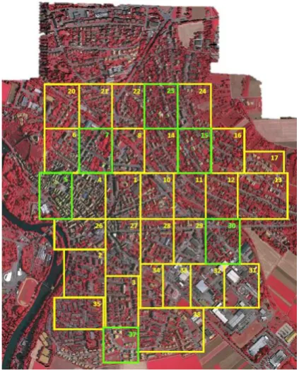
The ISPRS Benchmark Test on Urban Object Detection and Re-construction1introduced the Vaihingen dataset and made it pub-licly available. It contains 33 aerial images of the town of Vai-hingen in Baden-W¨urttemberg, Germany (see Figure 1). Each image has a resolution of roughly 2,000 by 2,000 pixels and a ground sampling distance (GSD) of 9 cm. For each pixel there are intensity values for three channels: near infrared, red, and green. Height information acquired by a LiDAR scanner is also available, but not used in this work. Ground truth is provided for 16 areas and has five classes (Car, Tree, Low vegetation, Build-ing, Impervious surfaces). Additionally there is a rejection class (Clutter / Background) which captures pixels not belonging to any of the five main classes so that every pixel has a ground truth value. A second set of ground truth data contains a 3 pixels wide border between sections of different classes. The reasoning be-ing that those pixels, in areas where two materials meet, very likely contain spectra from both. Those pixels can interrupt the learning process. To handle these separately, they form a sixth class: border. Table 4 gives an overview of all chosen areas. For completeness the Brutisellen dataset used in (Munoz-Mari et al., 2012) is included.
4. RESULTS AND DISCUSSION
This section reports and discusses the results of the experiments presented in the previous section.
1
The Vaihingen data set was provided by the German Society for Photogrammetry, Remote Sensing and Geoinformation (DGPF) (Cramer,
Experiment α Border B Dataset
1 - - - Brutisellen, Vaihingen #7
2 {0, 0.1, 0.25, 0.4} w/ 5000 Vaihingen #7
3 0.25 {w/, w/o} 5000 Vaihingen #7
4 0.25 w/ {2500, 5000, 7500} Vaihingen #7
5 0.25 w/ 5000 Vaihingen #{5, 7, 15, 23, 30, 37}
Table 3. Overview of the different parameter variations for the five experiments. Experiments 1-4 were also executed on the other selected areas of the Vaihingen dataset with very similar results. Therefore only area #7 is reported.
Dataset Sensor Spectral
bands GSD [m] Pixel count Classes Class distribution
Brutisellen QuickBird 4 2.40 40,762 9
Vaihingen (#5) Intergraph/ZI DMC 3 0.09 4,825,059 6
Vaihingen (#7) Intergraph/ZI DMC 3 0.09 4,825,059 6
Vaihingen (#15) Intergraph/ZI DMC 3 0.09 4,916,019 6
Vaihingen (#23) Intergraph/ZI DMC 3 0.09 4,838,646 6
Vaihingen (#30) Intergraph/ZI DMC 3 0.09 4,956,842 6
Vaihingen (#37) Intergraph/ZI DMC 3 0.09 3,982,020 6
Table 4. Overview of the different datasets. All datasets are aerial images of urban areas. Pixel counts are without background. Classes in Brutisellen: residential, commercial, vegetation, soil, bare soil, roads, pools, parkings, vegetation2. Classes in Vaihingen:
impervious surfaces, building, low vegetation, tree, car, border.
Figure 1. Overview of all 33 tiles of the Vaihingen dataset. Marked in green are the areas chosen for this work. Criteria for
the choice were: ground truth available, distributed over whole area, representing different characteristics from the whole
dataset (ratio of residential/industrial/vegetation).
4.1 Reproducing
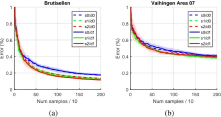
We were able to reproduce the results from (Munoz-Mari et al., 2012) for the Brutisellen dataset. Though we arrived at a final er-ror of 12% instead of 8%, we observed the same effects regarding the effectiveness of the active learning strategies, see Figure 2(a). These improve the learning rate and lead to a lower overall classi-fication error compared to random sampling strategies. Applying the same method to area 7 of the Vaihingen dataset leads to less definitive results, see Figure 2(b). Active learning still outper-forms the random sampling strategies, but by a smaller margin. This is a sign that the classification of this dataset is much more challenging. The main reason is that it has only three spectral bands (which is 25% fewer than Brutisellen). Another source for complications could be the much higher spatial resolution of this dataset because this requires a different weighting between spectral and spatial features. Furthermore the number of pixels in the Vaihingen dataset is 100 times greater. If the fixed number of bisecting iterations leads to an inadequate granularity of the clustering hierarchy is tested in experiment 3 (see 4.4).
As reported in (Munoz-Mari et al., 2012) the active strategies s1, s2, d1 outperform the random strategiess0, d0 because they
actively focus on the most uncertain leafs. On the Vaihingen dataset strategy (s1, d1) delivered slightly more consistent results
and is therefore chosen for the remainder of the experiments.
4.2 Removing outliers
0 50 100 150 200
Num samples / 10
0
Num samples / 10
0
Figure 2. Reproduction of the results from (Munoz-Mari et al., 2012) for the Brutisellen dataset (a). The result is the same as originally reported, though the final classification error was 12% in our case instead of 8%. The active strategies s1 and s2 clearly outperform the random sampling strategy s0. Applied to area 7 of the Vaihingen dataset, the results are not as distinct, but active
learning is still better (b).
0 500 1000 1500 2000
Number of Queries
Removed Fraction of Outliers (Area 07)
0.0 0.1 0.25 0.4
(a)
1000 1200 1400 1600 1800 2000
Number of Queries
Removed Fraction of Outliers (Area 07)
0.0 0.1 0.25 0.4
(b)
Figure 3. Removing varying fractions of pixels that are considered outliers (largest distance to the mean) has a small but
noticeable effect on the classification error. The right figure is a closeup of later iterations. The standard deviations are not
shown to provide a less cluttered image.
see Figure 3. This is a sign that the segments contain some outliers which negatively affect the mean. But removing more than 25% of the pixels does not affect the classification error fur-ther. Other possibilities of removing outliers can be considered in future work. For example using the median, removing out-liers based on pixels with high gradients, or assuming a normal distribution and a cutoff threshold based on its standard devia-tion. After evaluating these results we chose a moderate amount ofα= 0.25to remove.
4.3 Removing border class
The results are an almost halved classification error in area 7 and 25% reduced error in area 30, see Figure 4. The red curves are the original pixel based method, the blue curves are our proposed method based on the SLIC segmentation. The solid lines show the results of including border pixels whereas the dashed lines are from excluding them before clustering. The main contribut-ing factor is the handlcontribut-ing of mixed pixels by our method. This is also the reason why our method does not profit as much as the original method from removing the class of border pixels be-forehand. The learning curve of the Pixel w/o border case is de-creasing faster than the case Pixel w/ border, but not reaching the quality of the SLIC versions. This suggests that there is less noise in the clustering (it is lower than the w/ border case), but much information is “hidden” in the leafs of the tree.
0 500 1000 1500 2000
Number of Queries
0 500 1000 1500 2000
Number of Queries
Figure 4. Results of extending active queries with the proposed local segmentation for area 7 (a) and 30 (b) of the Vaihingen
dataset. The red learning curves (“Pixel”) are achieved by applying the original active query method directly on the pixels
of the image. The blue curves (“SLIC”) are achieved when the proposed extension is used with the SLIC algorithm. The dashed
lines are the results of removing mixed pixels from the border regions beforehand.
0 500 1000 1500 2000
Number of Queries
Number of Bisections (Area 07)
2,500 5,000 7,500
(a)
1500 1600 1700 1800 1900 2000
Number of Queries
Number of Bisections (Area 07)
2,500 5,000 7,500
(b)
Figure 5. Varying the number of bisections in the hierarchical clustering step leads to no significant change (less than 0.4
percent points) in classification error.
4.4 Number of bisections
The number of bisecting iterations in the clustering step is limited and remaining elements are grouped together in the leafs of the tree. Increasing the number of bisections leads to a deeper tree which increases the computation time for all following steps, yet there is no significant effect (less than 1% or 0.4 percent points) on the classification error, see Figure 5.
Figure 6. Detail of the SLIC segmentation result. The oversegmentation is advantageous because the segments can be
grouped together later in the clustering step, but undersegmentation cannot be corrected.
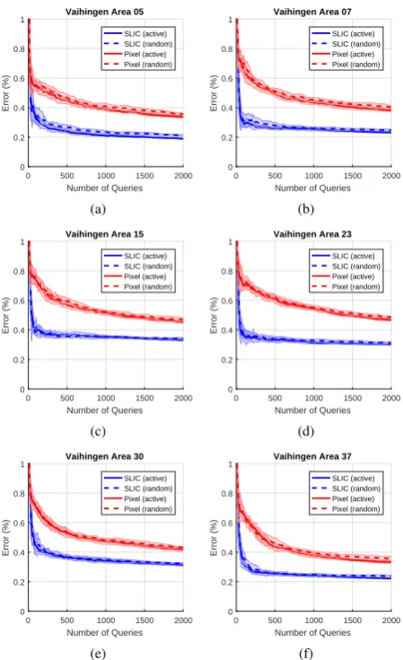
4.5 Different datasets
The results on the different datasets are very similar, see Figure 7. All show a large reduction of the classification error if the pro-posed method is used. This improvement is based on the remov-ing of mixed pixels which otherwise would lead to a clusterremov-ing inconsistent with the ground truth. This cannot be fixed by label-ing more samples and is the reason the classification error does not improve much further after 1,000 queries are reached. With the proposed method on the other hand, the clustering fits much better to the ground truth. Then even a few labeled samples are enough to reach a low classification error.
The use of the active learning strategy(s1, d1)also improves the
classification error compared to random sampling, but has a lot less influence than the use of the additional segmentation step. The reason for this is that active learning cannot compensate for noise in the clustering. This is a disadvantage of the proposed method. A solution could be an update of the clustering hierar-chy after more information, by querying labels from the user, is available.
4.6 General results
Visualizing the specific samples that were queried is a valuable tool in analyzing active learning algorithms. Since there is only a minor difference between active and random sampling in the presented method, this tool cannot be applied here. The selec-tion patterns are visually indistinguishable and therefore are not reported here.
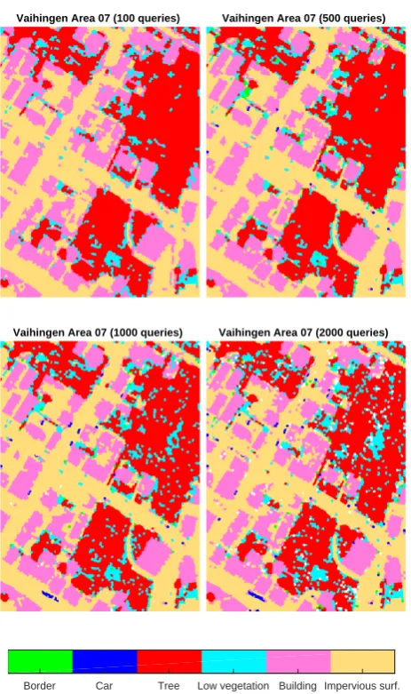
The resulting classification maps at different stages of the learn-ing process are displayed in Figure 8. In early stages (100 queries) not all classes are discovered. This is a sign of missing diversity during the selection process. This should be addressed by incor-porating a penalty for querying in already known areas into the selection strategies. After 500 queries there are not many changes observable which matches the learning curves in Figure 7.
5. CONCLUSION
This paper presented an extension to the active queries method by adding a new first step of local segmentation. The results were a drop in the overall classification error and an increased learning rate that is reaching certain classification quality with fewer labeled samples. This was achieved by replacing the seg-ments generated by the SLIC algorithm with representative pix-els. The cause of this effect is that mixed pixels are inherently
0 500 1000 1500 2000
Number of Queries
0 500 1000 1500 2000
Number of Queries
0 500 1000 1500 2000
Number of Queries
0 500 1000 1500 2000
Number of Queries
0 500 1000 1500 2000
Number of Queries
0 500 1000 1500 2000
Number of Queries
Figure 7. Comparison of the original pixel based active queries method (red) and the presented extension based on the SLIC algorithm (blue). Also shown is a comparison between random
sampling (dashed lines) and active learning (solid lines). Both active learning and the handling of mixed pixels improve the classification error, but the extraction of representative pixels far
Vaihingen Area 07 (100 queries) Vaihingen Area 07 (500 queries)
Vaihingen Area 07 (1000 queries) Vaihingen Area 07 (2000 queries)
Border Car Tree Low vegetation Building Impervious surf.
Figure 8. Classification maps at different stages of the learning process. At 100 queries not all classes are discovered. At 500 queries all classes are present and the result looks much like the
final result. Between 1,000 and 2,000 queries are not many changes which matches the observations from the learning
curves.
uncertain and hinder the learning process. Therefore, removing them speeds up the learning rate. A similar, but less pronounced, effect was achieved by removing mixed pixels from the dataset entirely. This was possible because the Vaihingen dataset pro-vides suitable ground truth. Since not all datasets offer this, the proposed extension is a helpful tool in handling mixed pixels in remote sensing data.
Our experiences with the SLIC algorithm show that it is very easy to handle. An advantage is the deterministic behavior, which ensures reproducible results. The regular structure of the seed points and missing merging of segments lead to oversegmenta-tion. In the presented method this is beneficial, but in other con-texts it could be a downside. To use it with hyperspectral images, either its combined Euclidean distance measure needs to be ex-tended or a preprocessing step to mitigate nonlinearities like in (Gross et al., 2015) can be applied.
The bisectingk-means algorithm is a very good choice because it leads to a natural hierarchical clustering of the data. A downside is the random initialization. This requires repeated execution to get reliable results. A deterministic variant might be easier to study and lead to more insights.
Overall, the active queries method is a very beneficial tool to in-corporate active learning into remote sensing classification tasks. It is easily adaptable to different strategies and extensions.
REFERENCES
Achanta, R., Shaji, A., Smith, K., Lucchi, A., Fua, P. and Susstrunk, S., 2012. Slic superpixels compared to state-of-the-art superpixel methods. IEEE Transactions on Pattern Analysis
and Machine Intelligence34(11), pp. 2274–2282.
Anderson, J. R., 1976.A Land Use and Land Cover Classification
System for Use with Remote Sensor Data. Geological Survey
professional paper, U.S. Government Printing Office.
Atlas, L. E., Cohn, D. and Ladner, R., 1990. Training connection-ist networks with queries and selective sampling. In:Advances in
Neural Information Processing Systems, Morgan Kaufmann, San
Mateo, Calif, pp. 566–573.
Balcan, M. F., Beygelzimer, A. and Langford, J., 2006. Agnostic active learning. In:International Conference on Machine Learn-ing, pp. 65–72.
Bruzzone, L. and Carlin, L., 2006. A multilevel context-based system for classification of very high spatial resolution images.
IEEE Transactions on Geoscience and Remote Sensing 44(9),
pp. 2587–2600.
Bruzzone, L. and Persello, C., 2010. Recent trends in classifica-tion of remote sensing data: active and semisupervised machine learning paradigms. In: International Geoscience and Remote
Sensing Symposium, IEEE, pp. 3720–3723.
Cheng, J. and Wang, K., 2007. Active learning for image retrieval with co-svm.Pattern Recognition40(1), pp. 330–334.
Cramer, M., 2010. The dgpf-test on digital airborne camera eval-uation overview and test design. PFG Photogrammetrie,
Cui, B., Lin, H. and Yang, Z., 2009. Uncertainty sampling-based active learning for protein–protein interaction extraction from biomedical literature. Expert Systems with Applications36(7), pp. 10344–10350.
Dasgupta, S. and Hsu, D. J., 2008. Hierarchical sampling for ac-tive learning. In:International Conference on Machine Learning, pp. 208–215.
Demir, B., Bovolo, F. and Bruzzone, L., 2012. Detection of land-cover transitions in multitemporal remote sensing images with active-learning-based compound classification. IEEE
Transac-tions on Geoscience and Remote Sensing50(5), pp. 1930–1941.
Di Gregorio, A. and Jansen, L. J. M., 2000. Land cover classifi-cation systems (LCCS): Classificlassifi-cation concepts and user manual. Food and Agriculture Organization of the United Nations, Rome.
Fleming, M. D., Berkebile, J. S. and Hoffer, R. M., 1975. Computer-aided analysis of landsat-1 mss data: A comparison of three approaches, including a ’modified clustering’ approach. Technical report, Purdue University.
Gross, W., Wuttke, S. and Middelmann, W., 2015. Transforma-tion of hyperspectral data to improve classificaTransforma-tion by mitigating nonlinear effects. In:Proceedings WHISPERS.
Hanneke, S., 2014. Theory of active learning. Technical report, Private.
Harak´e, L., Schilling, H., Blohm, C., Hillemann, M., Lenz, A., Becker, M., Keskin, G. and Middelmann, W., 2016. Concept for an airborne real-time isr system with multi-sensor 3d data acqui-sition. In: Optical Engineering + Applications, SPIE Proceed-ings, SPIE, p. 998709.
Hasanzadeh, M. and Kasaei, S., 2010. A multispectral image segmentation method using size-weighted fuzzy clustering and membership connectedness.IEEE Geoscience and Remote Sens-ing Letters7(3), pp. 520–524.
Huo, L.-Z., Tang, P., Zhang, Z. and Tuia, D., 2015. Semisuper-vised classification of remote sensing images with hierarchical spatial similarity. IEEE Geoscience and Remote Sensing Letters
12(1), pp. 150–154.
K¨a¨ari¨ainen, M., 2006. Active learning in the non-realizable case.
In:Algorithmic Learning Theory: Proceedings, Lecture Notes in
Computer Science, Vol. 4264, pp. 63–77.
Kashef, R. and Kamel, M. S., 2009. Enhanced bisecting -means clustering using intermediate cooperation. Pattern Recognition
42(11), pp. 2557–2569.
Krempl, G., Kottke, D. and Lemaire, V., 2015. Optimised prob-abilistic active learning (opal). Machine Learning 100(2-3), pp. 449–476.
Lee, S., 2004. Efficient multistage approach for unsupervised image classification. In: International Geoscience and Remote
Sensing Symposium: Proceedings, pp. 1581–1584.
Lee, S. and Crawford, M. M., 2004. Hierarchical clustering approach for unsupervised image classification of hyperspectral data. In:International Geoscience and Remote Sensing Sympo-sium: Proceedings, pp. 941–944.
Lee, S. and Crawford, M. M., 2005. Unsupervised multistage image classification using hierarchical clustering with a bayesian similarity measure. IEEE Transactions on Image Processing
14(3), pp. 312–320.
Liu, R., Wang, Y., Baba, T., Masumoto, D. and Nagata, S., 2008. Svm-based active feedback in image retrieval using clustering and unlabeled data.Pattern Recognition41(8), pp. 2645–2655.
Marcal, A. R. S. and Castro, L., 2005. Hierarchical clustering of multispectral images using combined spectral and spatial criteria.
In: International Geoscience and Remote Sensing Symposium:
Proceedings, Vol. 2, pp. 59–63.
Munoz-Mari, J., Tuia, D. and Camps-Valls, G., 2012. Semisuper-vised classification of remote sensing images with active queries.
IEEE Transactions on Geoscience and Remote Sensing50(10),
pp. 3751–3763.
Pasolli, E. and Melgani, F., 2010. Active learning methods for electrocardiographic signal classification. IEEE transactions on information technology in biomedicine : a publication of
the IEEE Engineering in Medicine and Biology Society14(6),
pp. 1405–1416.
Patra, S. and Bruzzone, L., 2011. A fast cluster-assumption based active-learning technique for classification of remote sensing im-ages. IEEE Transactions on Geoscience and Remote Sensing
49(5), pp. 1617–1626.
Schindler, K., 2012. An overview and comparison of smooth la-beling methods for land-cover classification. IEEE Transactions
on Geoscience and Remote Sensing50(11), pp. 4534–4545.
Senthilnath, J., Omkar, S. N., Mani, V., Diwakar, P. G. and Shenoy B, A., 2012. Hierarchical clustering algorithm for land cover mapping using satellite images. IEEE Journal of Selected
Topics in Applied Earth Observations and Remote Sensing5(3),
pp. 762–768.
Settles, B., 2012. Active Learning. Synthesis Lectures on Artifi-cial Intelligence and Machine Learning, Vol. 6, Morgan & Clay-pool Publishers.
Tuia, D., Mu˜noz-Mar´ı, J. and Camps-Valls, G., 2012. Remote sensing image segmentation by active queries. Pattern Recogni-tion45(6), pp. 2180–2192.
Tuia, D., Volpi, M., Copa, L., Kanevski, M. F. and Munoz-Mari, J., 2011. A survey of active learning algorithms for supervised remote sensing image classification. IEEE Journal of Selected Topics in Signal Processing5(3), pp. 606–617.
Wassenberg, J., Middelmann, W. and Sanders, P., 2009. An ef-ficient parallel algorithm for graph-based image segmentation.
In: Computer Analysis of Images and Patterns: Proceedings,
Springer Berlin Heidelberg, Berlin, Heidelberg, pp. 1003–1010.
Wuttke, S., Middelmann, W. and Stilla, U., 2015. Concept for a compound analysis in active learning for remote sensing. In:The International Archives of the Photogrammetry, Remote Sensing
and Spatial Information Sciences, Vol. XL-3/W2, pp. 273–279.
Zhang, D., Wang, F., Shi, Z. and Zhang, C., 2008. Localized con-tent based image retrieval by multiple instance active learning. In: