SEMANTIC3D.NET: A NEW LARGE-SCALE POINT CLOUD CLASSIFICATION
BENCHMARK
Timo Hackela, Nikolay Savinovb, Lubor Ladickyb, Jan D. Wegnera, Konrad Schindlera, Marc Pollefeysb
a
IGP, ETH Zurich, Switzerland - (timo.hackel, jan.wegner, konrad.schindler)@geod.baug.ethz.ch bCVG, ETH Zurich, Switzerland - (nikolay.savinov, lubor.ladicky, marc.pollefeys)@inf.ethz.ch
Commission II, WG II/6
ABSTRACT:
This paper presents a new 3D point cloud classification benchmark data set with over four billion manually labelled points, meant as input for data-hungry (deep) learning methods. We also discuss first submissions to the benchmark that use deep convolutional neural networks (CNNs) as a work horse, which already show remarkable performance improvements over state-of-the-art. CNNs have become the de-facto standard for many tasks in computer vision and machine learning like semantic segmentation or object detection in images, but have no yet led to a true breakthrough for 3D point cloud labelling tasks due to lack of training data. With the massive data set presented in this paper, we aim at closing this data gap to help unleash the full potential of deep learning methods for 3D labelling tasks. Oursemantic3D.netdata set consists of dense point clouds acquired with static terrestrial laser scanners. It contains 8semantic classes and covers a wide range of urban outdoor scenes: churches, streets, railroad tracks, squares, villages, soccer fields and castles. We describe our labelling interface and show that our data set provides more dense and complete point clouds with much higher overall number of labelled points compared to those already available to the research community. We further provide baseline method descriptions and comparison between methods submitted to our online system. We hopesemantic3D.netwill pave the way for deep learning methods in 3D point cloud labelling to learn richer, more general 3D representations, and first submissions after only a few months indicate that this might indeed be the case.
1. INTRODUCTION
Deep learning has made a spectacular comeback since the semi-nal paper of (Krizhevsky et al., 2012), which revives earlier work of (Fukushima, 1980, LeCun et al., 1989). Especially deep con-volutional neural networks (CNN) have quickly become the core technique for a whole range of learning-based image analysis tasks. The large majority of state-of-the-art methods in computer vision and machine learning include CNNs as one of their essen-tial components. Their success for image-interpretation tasks is mainly due to (i) easily parallelisable network architectures that facilitate training from millions of images on a single GPU and (ii) the availability of huge public benchmark data sets like Im-ageNet(Deng et al., 2009, Russakovsky et al., 2015) and Pas-cal VOC(Everingham et al., 2010) for rgb images, orSUN rgb-d(Song et al., 2015) for rgb-d data.
While CNNs have been a great success story for image interpre-tation, it has been less so for 3D point cloud interpretation. What makes supervised learning hard for 3D point clouds is the sheer size of millions of points per data set, and the irregular, not grid-aligned, and in places very sparse structure, with strongly varying point density (Figure 1).
While recording is nowadays straight-forward, the main bottle-neck is to generate enough manually labeled training data, needed for contemporary (deep) machine learning to learn good models, which generalize well across new, unseen scenes. Due to the ad-ditional dimension, the number of classifier parameters is larger in 3D space than in 2D, and specific 3D effects like occlusion or variations in point density lead to many different patterns for identical output classes. This aggravates training good, general classifiers and we generally need more training data in 3D than in 2D1. In contrast to images, which are fairly easy to annotate even
1
Note that the large number of 3D points ofsemantic3d.net(4×10⁹ points) is at the same scale as the number of pixels of theSUN rgb-d benchmark (≈ 3.3×10⁹
px) (Song et al., 2015), which aims at 3D
for untrained users, 3D point clouds are harder to interpret. Nav-igation in 3D is more time-consuming and the strongly varying point density aggravates scene interpretation.
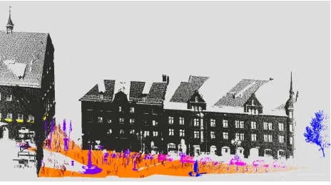
Figure 1: Example point cloud of the benchmark dataset, where colours indicate class labels.
In order to accelerate the development of powerful algorithms for point cloud processing2, we provide the (to our knowledge) hitherto largest collection of (terrestrial) laser scans with point-level semantic ground truth annotation. In total, it consists of over4·109
points and class labels for8classes. The data set is split into training and test sets of approximately equal size. The scans are challenging, not only due to their size of up to≈4·108 points per scan, but also because of their high measurement res-olution and long measurement range, leading to extreme density
object classification. However, the number of 3D points per laser scan (≈4×10⁸
points) is much larger than the number of pixels per image (≈4×105px).
2
Note that, besides laser scanner point clouds, it is also more efficient to classify point clouds generated from SfM pipelines directly instead of going through all individual images to then merge results (Riemenschnei-der et al., 2014).
This contribution has been peer-reviewed. The double-blind peer-review was conducted on the basis of the full paper.
changes and large occlusions. For convenient use of the bench-mark test we provide not only freely available data, but also an automated online submission system as well as public results of the submitted methods. The benchmark also includes baselines, one following the standard paradigm of eigenvalue-based feature extraction at multiple scales followed by classification with a ran-dom forest, the other a basic deep learning approach. Moreover, first submissions have been made to the benchmark, which we also briefly discuss.
2. RELATED WORK
Benchmarking efforts have a long tradition in the geospatial data community and particularly in ISPRS. Recent efforts include, for example, theISPRS-EuroSDR benchmark on High Density Aerial Image Matching3 that aims at evaluating dense matching meth-ods for oblique aerial images (Haala, 2013, Cavegn et al., 2014) and theISPRS Benchmark Test on Urban Object Detection and Reconstruction, which contains several different challenges like semantic segmentation of aerial images and 3D object reconstruc-tion (Rottensteiner et al., 2013).
In computer vision, very large-scale benchmark data sets with millions of images have become standard for learning-based im-age interpretation tasks. A variety of datasets have been intro-duced, many tailored for a specific task, some serving as basis for annual challenges for several consecutive years (e.g.,ImageNet, Pascal VOC). Datasets that aim at boosting research in image classification and object detection heavily rely on images down-loaded from the internet. Web-based imagery has been a major driver of benchmarks because no expensive, dedicated photogra-phy campaigns have to be accomplished for dataset generation. This enables scaling benchmarks from hundreds to millions of images, although often weakly annotated and with a considerable amount of label noise that has to be taken into account. Addi-tionally, one can assume that internet images constitute a very general collection of images with less bias towards particular sen-sors, scenes, countries, objects etc., which allows training richer models that generalize well.
One of the first successful attempts to object detection in im-ages at very large scale istinyimageswith over 80 million small (32×32px) images (Torralba et al., 2008). A milestone and still widely used dataset for semantic image segmentation is the famous Pascal VOC (Everingham et al., 2010) dataset and chal-lenge, which has been used for training and testing many of the well-known, state-of-the-art algorithms today like (Long et al., 2015, Badrinarayanan et al., 2015). Another, more recent dataset isMSCOCO4, which contains300,000images with annotations that allow for object segmentation, object recognition in context, and image captioning. One of the most popular benchmarks in computer vision today is theImageNetdataset (Deng et al., 2009, Russakovsky et al., 2015), which made Convolutional Neural Networks popular in computer vision (Krizhevsky et al., 2012). It contains>14×106
images organized according to the Word-Net hierarchy5, where words are grouped into sets of cognitive synonyms.
The introduction of the popular, low-cost gaming device Microsoft Kinect gave rise to several, large rgb-d image databases. Popular examples are theNYU Depth Dataset V2(Silberman et al., 2012) or SUN RGB-D(Song et al., 2015) that provide labeled rgb-d
3
images for object segmentation and scene understanding. Com-pared to laser scanners, low-cost, structured-light rgb-d sensors have much shorter measurement ranges, lower resolutions, and work poorly outdoors due to interference of the infrared spectrum of the sunlight with the projected sensor pattern.
To the best of our knowledge, no publicly available dataset with laser scans at the scale of the aforementioned vision benchmarks exists today. Thus, many recent Convolutional Neural Networks that are designed for Voxel Grids (Brock et al., 2017, Wu et al., 2015) resort to artificially generated data from the CAD models of ModelNet (Wu et al., 2015), a rather small, synthetic dataset. As a consequence, recent ensemble methods (e.g., (Brock et al., 2017)) reach performance of over97%on ModelNet10, which clearly indicates a model overfit due to limited data.
Those few existing laser scan datasets are mostly acquired with mobile mapping devices or robots likeDUT1(Zhuang et al., 2014),
DUT2(Zhuang et al., 2015), orKAIST(Choe et al., 2013), which are small (< 107
points) and not publicly available. Publicly availabe laser scan datasets include theOakland dataset(Munoz et al., 2009) (< 2×10⁶
points), theSydney Urban Objects data set(De Deuge et al., 2013), theParis-rue-Madame database
(Serna et al., 2014) and data from theIQmulus & TerraMobilita Contest(Vallet et al., 2015). All have in common that they use 3D LIDAR data from a mobile mapping car which provides a much lower point density than a typical static scan, like ours. They are also relatively small, such that supervised learning al-gorithms easily overfit. The majority of today’s available point cloud datasets comes without a thorough, transparent evaluation that is publicly available on the internet, continuously updated and that lists all submissions to the benchmark.
With thesemantic3D.netbenchmark presented in this paper, we aim at closing this gap. It provides the largest labeled 3D point cloud data set with approximately four billion hand-labeled points, comes with a sound evaluation, and continuously updates submis-sions. It is the first dataset that allows full-fledged deep learning on real 3D laser scans that have high-quality, manually assigned labels per point.
3. OBJECTIVE
Given a set of points (here: dense scans from a static, terres-trial laser scanner), we want to infer one individual class label per point. We provide three baseline methods that are meant to represent typical categories of approaches recently used for the task.
i) 2D image baseline:
Many state-of-the-art laser scanners also acquire color values or even entire color images for the scanned scene. Color images can add additional object evidence that may help classification. Our first, naive baseline classifies only the 2D color images without using any depth information, so as to establish a link to the vast literature on 2D semantic image segmentation. Modern meth-ods use Deep Convolutional Neural Networks as a workhorse. Encoder-decoder architectures, like SegNet (Badrinarayanan et al., 2015), are able to infer the labels of an entire image at once. Deep architectures can also be combined with Conditional Ran-dom Fields (CRF) (Chen et al., 2016). Our baseline method in Section 3.1 covers image-based semantic segmentation.
ii) 3D Covariance baseline: A more specific approach, which takes advantage of the 3D information, is to work on point clouds ISPRS Annals of the Photogrammetry, Remote Sensing and Spatial Information Sciences, Volume IV-1/W1, 2017
Figure 2:Top row:projection of ground truth to images.Bottom row:results of classification with the image baseline.White:unlabeled pixels,black:pixels with no corresponding 3D point,gray:buildings,orange:man made ground,green:natural ground,yellow:low vegetation,blue:high vegetation,purple: hard scape,pink:cars
directly. We use a recent implementation of the standard classifi-cation pipeline, i.e., extract hand-crafted features from 3D (multi-scale) neighbourhoods, and feed them to a discriminative learn-ing algorithm. Typical features encode surface properties based on the covariance tensor of a point’s neighborhood (Demantk´e et al., 2011) or a randomized set of histograms (Blomley et al., 2014). Additionally, height distributions can be encoded by us-ing cylindrical neighborhoods (Monnier et al., 2012, Weinmann et al., 2013). The second baseline method (Section 3.2) repre-sents this category.
iii) 3D CNN baseline: It is a rather obvious extension to apply deep learning also to 3D point clouds, mostly using voxel grids to obtain a regular neighbourhood structure. To work efficiently with large point neighborhoods in clouds with strongly varying density, recent work uses adaptive neighbourhood data structures like octrees (Wu et al., 2015, Brock et al., 2017, Riegler et al., 2017) or sparse voxel grids (Engelcke et al., 2017). Our third baseline method in Section 3.3 is a basic, straight-forward imple-mentation of 3D voxel-grid CNNs.
3.1 2D Image Baseline
We convert color values of the scans to separate images (without depth) with cube mapping (Greene, 1986). Ground truth labels are also projected from the point clouds to image space, such that the 3D point labeling task turns into a pure semantic image seg-mentation problem of 2D RGB images (Figure 2). We chose the associate hierarchical fields method (Ladicky et al., 2013) for se-mantic segmentation because it has proven to deliver good perfor-mance for a variety of tasks (e.g., (Montoya et al., 2014, Ladick´y et al., 2014)) and was available in its original implementation.
The method works as follows: four different types of features – texton (Malik et al., 2001), SIFT (Lowe, 2004), local quantized ternary patters (Hussain and Triggs, 2012) and self-similarity fea-tures (Shechtman and Irani, 2007) – are extracted densely per im-age pixel. Each feature category is separately clustered into512 distinct patterns using standard K-means clustering, which corre-sponds to a typical bag-of-words representation. For each pixel in an image, the feature vector is a concatenation of bag-of-word
histograms over a fixed set of200rectangles of varying sizes. These rectangles are randomly placed in an extended neighbour-hood around a pixel. We use multi-class boosting (Torralba et al., 2004) as classifier and the most discriminative weak features are found as explained in (Shotton et al., 2006). To add local smooth-ing without loossmooth-ing sharp object boundaries, we smooth inside superpixels and favor class transitions at their boundaries. Super-pixels are extracted via mean-shift (Comaniciu and Meer, 2002) with 3 sets of coarse-to-fine parameters as described in (Ladicky et al., 2013). Class likelihoods of overlapping superpixels are predicted using the feature vector consisting of a bag-of-words representation of each superpixel. Pixel-based and superpixel-based classifiers with additional smoothness priors over pixels and superpixels are combined in a probabilistic fashion in a con-ditional random field framework as proposed in (Kohli et al., 2008). The most probable solution of the associative hierarchical optimization problem is found using the move making (Boykov et al., 2001) graph-cut based algorithm (Boykov and Kolmogorov, 2004), with appropriate graph construction for higher-order po-tentials (Ladicky et al., 2013).
3.2 3D Covariance Baseline
The second baseline was inspired by (Weinmann et al., 2015). It infers the class label directly from the 3D point cloud using multiscale features and discriminative learning. Again, we had access to the original implementation. That method uses an ef-ficient approximation of multi-scale neighbourhoods, where the point cloud is sub-sampled into a multi-resolution pyramid, such that a constant, small number of neighbours per level captures the multi-scale information. The multi-scale pyramid is generated by voxel-grid filtering with uniform spacing.
The feautre set extracted at each level is an extension of the one decribed in (Weinmann et al., 2013). It uses different combina-tions of eigenvalues and eigenvectors of the covariance per point-neighborhood to different geometric surface properties. Further-more, height features based on vertical, cylindrical neighbour-hoods are added to emphasize the special role of the gravity di-rection (assuming that scans are, as usual, aligned to the vertical).
This contribution has been peer-reviewed. The double-blind peer-review was conducted on the basis of the full paper.
Note that we do not make use of color values or scanner intensi-ties. These are not always available in point clouds, and we em-pirically found that they do not improve the results of the method. As classifier, we use a random forest, where optimal parameters are found with grid search and five fold cross-validation. Please refer to (Hackel et al., 2016) for details.
3.3 3D CNN Baseline
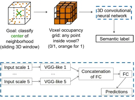
We design our baseline for the point cloud classification task fol-lowing recent VoxNet (Maturana and Scherer, 2015) and ShapeNet (Wu et al., 2015) 3D encoding ideas. The pipeline is illustrated in Fig. 3. Instead of generating a global 3D voxel-grid prior to pro-cessing, we create16×16×16voxel cubes per scan point6. We
Figure 3: Our deep neural network pipeline.
do this at5different resolutions, where voxel size ranges from 2.5cm to40cm (multiplied by powers of2) and encode empty voxel cells as0and filled ones as1. The input to the CNN is thus encoded in a multidimensional tensor with5×16×16×16cube entries per scan point.
Each of the five scales is handled separately by a VGG-like net-work path which includes convolutional, pooling and ReLU lay-ers. The5separate network paths are finally concatenated into a single representation, which is passed through two fully-connected layers. The output of the second fully-connected layer is an8 -dimensional vector, which contains the class scores for each of the8classes in this benchmark challenge. Scores are transformed to class conditional probabilities with the soft-max function.
Before describing the network architecture in detail we introduce the following notation:
c(i, o)stands for convolutional layers with3×3×3filters,iinput channels,ooutput channels, zero-padding of size1at each border and a stride of size1.f(i, o)stands for fully-connected layers.r
stands for a ReLU non-linearity,mstands for a volumetric max pooling with receptive field2×2×2, applied with a stride of size 2in each dimension,dstands for a dropout with0.5probability,
sstands for a soft-max layer.
Our 3D CNN architecture assembles these components to a VGG-like network structure. We choose the filter size in convolutional layers as small as possible (3×3×3), as recommended in recent work (He et al., 2016), to have the least amount of parameters
6
This strategy automatically centers each voxel-cube per scan point. Note that for the alternative approach of a global voxel grid, several scan points could fall into the same grid cell in dense scan parts. This would require scan point selection per grid cell, which is computationally costly and results in (undesired) down-sampling.
per layer and, hence, reduce both the risk of overfitting and the computational cost.
For the5separate network paths that act on different resolutions, we use a VGG-like (Simonyan and Zisserman, 2014) architec-ture:
(c(1,16), r, m, c(16,32), r, m, c(32,64), r, m).
The output is vectorized, concatenated between scales and the two fully-connected layers are applied on top to predict the class responses:
(f(2560,2048), r, d, f(2048,8), s).
For training we deploy the standard multi-class cross-entropy loss. Deep learning is non-convex but it can be efficiently optimized with stochastic gradient descent (SGD), which produces clas-sifiers with state-of-the-art prediction performance. The SGD algorithm uses randomly sampled mini-batches of several hun-dred points per batch to iteratively update the parameters of the CNN. We use the popular adadelta algorithm (Zeiler, 2012) for optimization, an extension of stochastic gradient decent (Bottou, 2010).
We use a mini batch size of100training samples (i.e., points), where each batch is sampled randomly and balanced (contains equal numbers of samples per class). We run training for74,700 batches and sample training data from a large and representa-tive point cloud with 259million points (sg28 4). A standard pre-processing step for CNNs is data augmentation to enlarge the training set and to avoid overfitting. Here, we augment the train-ing set with a random rotation around the z-axis after every100 batches. During experiments it turned out that additional training data did not improve performance. This indicates that in our case we rather deal with underfitting (as opposed to overfitting), i.e. our model lacks the capacity to fully capture all the evidence in the available training data7. We thus refrain from further possible augmentations like randomly missing points or adding noise.
Our network is implemented in C++ and Lua and uses the Torch7 framework (Collobert et al., 2011) for deep learning. The code and the documentation for this baseline are publicly available at https://github.com/nsavinov/semantic3dnet.
4. DATA
Our30published terrestrial laser scans consist of in total≈4 bil-lion 3D points and contain urban and rural scenes, like farms, town halls, sport fields, a castle and market squares. We inten-tionally selected various different natural and man-made scenes to prevent over-fitting of the classifiers. All of the published scenes were captured in Central Europe and describe typical Eu-ropean architecture as shown in Figure 4. Surveying-grade laser scanners were used for recording these scenes. Colorization was performed in a post processing step by deploying a high reso-lution cubemap, which was generated from camera images. In general, static laser scans have a very high resolution and are able to measure long distances with little noise. Especially com-pared to point clouds derived via structure-from-motion pipelines or Kinect-like structured light sensors, laser scanners deliver su-perior data quality.
Scanner positions for data recording were selected as usually done in the field: only little scan overlap as needed for registration, so that scenes can be recorded in a minimum of time. This free
7
Note that our model reaches hardware limits of our GPU (TitanX with 12GB of RAM) and we thus did not experiment with larger networks at this point.
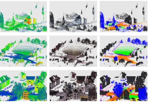
Figure 4: Intensity values (left), rgb colors (middle) and class labels (right) for example data sets.
choice of the scanning position implies that no prior assumption based on point density and on class distributions can be made. We publish up to3laser scans per scene that have small overlap. The relative position of laser scans at the same location was estimated from targets.
We use the following8classes within this benchmark challenge, which cover: 1)man made terrain: mostly pavement;2)natural terrain: mostly grass;3)high vegetation: trees and large bushes;
4)low vegetation: flowers or small bushes which are smaller than 2m;5)buildings: Churches, city halls, stations, tenements, etc.;
6)remaining hard scape: a clutter class with for instance gar-den walls, fountains, banks, etc.;7)scanning artifacts: artifacts caused by dynamically moving objects during the recording of the static scan;8)cars and trucks. Some of these classes are ill-defined, for instance some scanning artifacts could also go for cars or trucks and it can be hard to differentiate between large and small bushes. Yet, these classes can be helpful in numer-ous applications. Please note that in most applications class7, scanning artifacts, gets filtered with heuristic rule sets. Within this benchmark we want to deploy machine learning techniques instead, and thus do not perform any heuristic pre-processing.
In our view, large data sets are important for two reasons:a) Typ-ically, real world scan data sets are large. Hence, methods which have an impact on real problems have to be able to process a large amount of data.b)Large data sets are especially important when developing methods with modern inference techniques ca-pable of representation learning. With too small datasets, good results leave strong doubts about possible overfitting; unsatisfac-tory results, on the other hand, are hard to interpret as guidelines for further research: are the mistakes due to short-comings of the method, or simply caused by unsufficient training data?
4.1 Point Cloud Annotation
In contrast to common strategies for 3D data labelling that first compute an over-segmentation followed by segment-labeling, we manually assign each point a class label individually. Although this strategy is more labor-intensive, it avoids inheriting errors from the segmentation approach and, more importantly, classi-fiers do not learn hand-crafted rules of segmentation algorithms when trained with the data. In general, it is more difficult to label a point cloud by hand than images. The main problem is that it is hard to select a 3D point on a 2D monitor from a set of mil-lions of points without a clear neighbourhood/surface structure. We tested two different strategies:
Annotation in 3D: We follow an iterative filtering strategy, where we manually select a couple of points, fit a simple model to the data, remove the model outliers and repeat these steps until all in-liers belong to the same class. With this procedure it is possible to select large buildings in a couple of seconds. A small part of the point clouds was labeled with this approach by student assistants at ETH Zurich.
Annotation in 2D: The user rotates a point cloud, fixes a 2D view and draws a closed polygon which splits a point cloud into two parts (inside and outside of the polygon). One part usually contains points from the background and is discarded. This pro-cedure is repeated a few times until all remaining points belong to the same class. At the end all points are separated into different layers corresponding to classes of interest. This 2D procedure works well with existing software packages (Daniel Girardeau-Montaut, CloudCompare, 2016) such that it can be outsourced to external labelers more easily than the 3D work-flow. We used this procedure for all data sets where annotation was outsourced.
This contribution has been peer-reviewed. The double-blind peer-review was conducted on the basis of the full paper.
Method
IoU
OA
t
[
s
]
IoU
1IoU
2IoU
3IoU
4IoU
5IoU
6IoU
7IoU
8HarrisNet
0.623
0.881
unknown
0.818
0.737
0.742
0.625
0.927
0.283
0.178
0.671
DeepSegNet
0.516
0.884
unknown
0.894
0.811
0.590
0.441
0.853
0.303
0.190
0.050
TMLC-MS
0.494
0.850
38421
0.911
0.695
0.328
0.216
0.876
0.259
0.113
0.553
TML-PC
0.391
0.745
unknown
0.804
0.661
0.423
0.412
0.647
0.124
0.0*
0.058
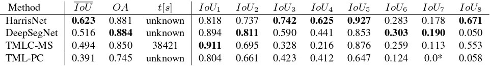
Table 1: Semantic3d benchmark results on the full data set: 3D covariance baselineTMLC-MS, 2D RGB image baselineTML-PC, and first submissionsHarrisNetandDeepSegNet.IoUfor categories (1) man-made terrain, (2) natural terrain, (3) high vegetation, (4) low vegetation, (5) buildings, (6) hard scape, (7) scanning artefacts, (8) cars. * Scanning artefacts were ignored for 2D classification because they are not present in the image data.
Method
IoU
OA
t
[
s
]
IoU
1IoU
2IoU
3IoU
4IoU
5IoU
6IoU
7IoU
8TMLC-MSR
0.542
0.862
1800
0.898
0.745
0.537
0.268
0.888
0.189
0.364
0.447
DeepNet
0.437
0.772
64800
0.838
0.385
0.548
0.085
0.841
0.151
0.223
0.423
TML-PCR
0.384
0.740
unknown
0.726
0.73
0.485
0.224
0.707
0.050
0.0*
0.15
Table 2: Semantic3d benchmark results on the reduced data set: 3D covariance baselineTMLC-MSR, 2D RGB image baseline TML-PCR, and our 3D CNN baselineDeepNet. TMLC-MSRis the same method asTMLC-MS, the same goes forTMLC-PCRand TMLC-PC. In both casesRindicates classifiers on the reduced dataset. IoUfor categories (1) man-made terrain, (2) natural terrain, (3) high vegetation, (4) low vegetation, (5) buildings, (6) hard scape, (7) scanning artefacts, (8) cars. * Scanning artefacts were ignored for 2D classification because they are not present in the image data.
5. EVALUATION
We follow Pascal VOC challenge’s (Everingham et al., 2010) choice of the main segmentation evaluation measure and use In-tersection over Union(IoU)8averaged over all classes. Assume classes are indexed with integers from{1, . . . , N}whereN is an overall number of classes. LetCbe anN×Nconfusion ma-trix of the chosen classification method, where each entrycijis a number of samples from ground-truth classipredicted as classj. Then the evaluation measure per classiis defined as
IoUi=
cii
cii+P j6=i
cij+P k6=i
cki
. (1)
The main evaluation measure of our benchmark is thus
IoU = N
P
i=1
IoUi
N . (2)
We also reportIoUifor each classiand overall accuracy
OA=
N
P
i=1
cii
N
P
j=1 N
P
k=1
cjk
(3)
as auxiliary measures and provide the confusion matrixC. Fi-nally, each participant is asked to specify the timeT it took to classify the test set as well as the hardware used for experiments. This measure is important for understanding how suitable the method is in real-world scenarios where usually billions of points are required to be processed.
For computational demanding methods we provide a reduced chal-lenge consisting of a subset of the published test data. The re-sults of our baseline methods as well as submissions are shown in Table 1 for the full challenge and in Table 2 for the reduced
8I oU
compensates for different class frequencies as opposed to, for example,overall accuracythat does not balance different class frequen-cies giving higher influence to large classes.
challenge. Of the three published baseline methods the covari-ance based method performs better than the CNN baseline and the color based method. Due to its computational cost we could only run our own deep learning baselineDeepNeton the reduced data set. We expect a network with higher capacity to perform much better. Results on the full challenge of two (unfortunately yet unpublished) 3D CNN methods,DeepSegNetandHarrisNet, already beat our covariance baseline by a significant margin (Ta-ble 1) of2respective12percent points. This indicates that deep learning seems to be the way to go also for point clouds, if enough data is available for training. It is a first sign that our benchmark already starts to work and generates progress.
6. BENCHMARK STATISTICS
Class distributions in test and training set are rather similar, as shown in Figure 5a. Interestingly, the class with most samples is
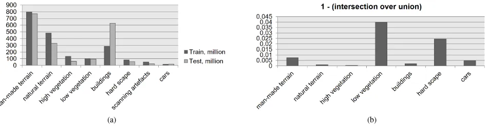
man-made terrainbecause, out of convenience, operators in the field tend to place the scanner on flat and paved ground. Re-call also the quadratic decrease of point density with distance to the scanner, such that many samples are close to the scanner. The largest difference between samples in test and training sets occurs for classbuilding. However, this does not seem to af-fect the performance of the submissions so far. Most difficult classes,scanning artefactsandcars, have only few training and test samples and a large variation of possible object shapes. Scan-ning artefactsis probably the hardest class because the shape of artefacts mostly depends on the movement of objects during the scanning process. Note that, following discussions with industry professionals, classhard scapewas designed as clutter class that contains all sorts of man-made objects except houses, cars and ground.
In order to get an intuition of the quality of the manually acquired labels, we also checked the label agreement among human anno-tators. This provides an indicative measure on how much dif-ferent annotators agree in labeling the data, and can be viewed as an internal check of manual labeling precision. We roughly estimate the label agreement of different human annotators in ar-eas where different scans of the same scene overlap. Because we cannot rule out completely that some overlapping areas might ISPRS Annals of the Photogrammetry, Remote Sensing and Spatial Information Sciences, Volume IV-1/W1, 2017
(a) (b)
Figure 5: (a) Number of points per class over all scans and (b) ground truth label errors estimated in overlapping parts of adjacent scans.
have been labeled by the same person (labeling was outsourced and we thus do not know exactly who annotated what), this can only be viewed as an indicative measure. Recall that overlaps of adjacent scans can precisely be established via artificial markers in the scene. Even if scan alignments would be perfect without any error, no exact point-to-point correspondences exist between two scans, because scan points acquired from two different loca-tions will never exactly fall onto the same spot. We thus have to resort to nearest neighbor search to find point correspondences. Moreover, not all scan points have a corresponding point in the adjacent scan. A threshold of5cm on the distance is used to ignore those points where no correspondence exists. Once point correspondences have been estblished, it is possible to transfer ground truth labels from one cloud to the other and compute a confusion matrix. Note that this definition of correspondence is not symmetric, point correspondences from cloud A in cloud B are not equal to correspondences of cloud B in cloud A. For each pair we calculate two intersection-over-union (IoUi) values which indicate a maximum label disagreement of<5%. No cor-respondences can be found on moving objects of course, hence we ignored categoryscanning artefactsin the evaluation in Fig-ure 5b.
7. CONCLUSION AND OUTLOOK
Thesemantic3D.netbenchmark provides a large set of high qual-ity terrestrial laser scans with over 4 billion manually annotated points and a standardized evaluation framework. The data set has been published recently and only has few submissions, yet, but we are optimistic this will change in the future. First submissions already show that finally CNNs are beginning to outperform more conventional approaches, for example our covariance baseline, on large 3D laser scans. Our goal is that submissions on this bench-mark will yield better comparisons and insights into the strengths and weaknesses of different classification approaches for point cloud processing, and hopefully contribute to guide research ef-forts in the longer term. We hope the benchmark meets the needs of the research community and becomes a central resource for the development of new, efficient and accurate methods for classifi-cation in 3D space.
ACKNOWLEDGEMENT
This work is partially funded by the Swiss NSF project 163910, the Max Planck CLS Fellowship and the Swiss CTI project 17136.1 PFES-ES.
REFERENCES
Badrinarayanan, V., Kendall, A. and Cipolla, R., 2015. Segnet: A deep convolutional encoder-decoder architecture for image seg-mentation. arXiv preprint arXiv:1511.00561.
Blomley, R., Weinmann, M., Leitloff, J. and Jutzi, B., 2014. Shape distribution features for point cloud analysis-a geometric histogram approach on multiple scales. ISPRS Annals of the Pho-togrammetry, Remote Sensing and Spatial Information Sciences.
Bottou, L., 2010. Large-scale machine learning with stochas-tic gradient descent. In: Proceedings of COMPSTAT’2010, Springer, pp. 177–186.
Boykov, Y. and Kolmogorov, V., 2004. An Experimental Com-parison of Min-Cut/Max-Flow Algorithms for Energy Minimiza-tion in Vision. TransacMinimiza-tions on Pattern Analysis and Machine Intelligence.
Boykov, Y., Veksler, O. and Zabih, R., 2001. Fast approximate energy minimization via graph cuts. PAMI.
Brock, A., Lim, T., Ritchie, J. and Weston, N., 2017. Genera-tive and discriminaGenera-tive voxel modeling with convolutional neural networks.
Cavegn, S., Haala, N., Nebiker, S., Rothermel, M. and Tutzauer, P., 2014. Benchmarking high density image matching for oblique airborne imagery. In: Int. Arch. Photogramm. Remote Sens. Spa-tial Inf. Sci., Vol. XL-3, pp. 45–52.
Chen, L.-C., Papandreou, G., Kokkinos, I., Murphy, K. and Yuille, A. L., 2016. Deeplab: Semantic image segmentation with deep convolutional nets, atrous convolution, and fully connected crfs. arXiv preprint arXiv:1606.00915.
Choe, Y., Shim, I. and Chung, M. J., 2013. Urban structure clas-sification using the 3d normal distribution transform for practical robot applications. Advanced Robotics 27(5), pp. 351–371.
Collobert, R., Kavukcuoglu, K. and Farabet, C., 2011. Torch7: A matlab-like environment for machine learning. In: BigLearn, NIPS Workshop.
Comaniciu, D. and Meer, P., 2002. Mean shift: A robust approach toward feature space analysis. PAMI.
Daniel Girardeau-Montaut, CloudCompare, 2016.http://www. danielgm.net/cc/.
De Deuge, M., Quadros, A., Hung, C. and Douillard, B., 2013. Unsupervised feature learning for classification of outdoor 3d scans. In: Australasian Conference on Robitics and Automation, Vol. 2.
Demantk´e, J., Mallet, C., David, N. and Vallet, B., 2011. Di-mensionality based scale selection in 3d lidar point clouds. The International Archives of Photogrammetry, Remote Sensing and Spatial Information Sciences.
Deng, J., Dong, W., Socher, R., Li, L.-J., Li, K. and Fei-Fei, L., 2009. Imagenet: A large-scale hierarchical image database. In: Computer Vision and Pattern Recognition, 2009. CVPR 2009. IEEE Conference on, IEEE, pp. 248–255.
Engelcke, M., Rao, D., Wang, D. Z., Tong, C. H. and Posner, I., 2017. Vote3deep: Fast object detection in 3d point clouds using efficient convolutional neural networks.
This contribution has been peer-reviewed. The double-blind peer-review was conducted on the basis of the full paper.
Everingham, M., van Gool, L., Williams, C., Winn, J. and Zisser-man, A., 2010. The pascal visual object classes (voc) challenge. International Journal of Computer Vision 88(2), pp. 303–338.
Fukushima, K., 1980. Neocognitron: A self-organizing neural network model for a mechanism of pattern recognition unaffected by shift in position. Biological cybernetics 36(4), pp. 193–202.
Greene, N., 1986. Environment mapping and other applications of world projections. IEEE Computer Graphics and Applications 6(11), pp. 21–29.
Haala, N., 2013. The landscape of dense image matching algo-rithms. In: Photogrammetric Week 13, pp. 271–284.
Hackel, T., Wegner, J. D. and Schindler, K., 2016. Fast semantic segmentation of 3D point clouds with strongly varying point den-sity. In: ISPRS Annals of the Photogrammetry, Remote Sensing and Spatial Information Sciences, Vol. III-3, pp. 177–184.
He, K., Zhang, X., Ren, S. and Sun, J., 2016. Deep residual learn-ing for image recognition. In: Proceedlearn-ings of the IEEE Confer-ence on Computer Vision and Pattern Recognition, pp. 770–778.
Hussain, S. and Triggs, B., 2012. Visual recognition using lo-cal quantized patterns. In: European Conference on Computer Vision.
Kohli, P., Ladicky, L. and Torr, P. H. S., 2008. Robust higher order potentials for enforcing label consistency. In: Conference on Computer Vision and Pattern Recognition.
Krizhevsky, A., Sutskever, I. and Hinton, G. E., 2012. Imagenet classification with deep convolutional neural networks.
Ladicky, L., Russell, C., Kohli, P. and Torr, P., 2013. Associative hierarchical random fields. PAMI.
Ladick´y, L., Zeisl, B. and Pollefeys, M., 2014. Discriminatively trained dense surface normal estimation. In: European Confer-ence on Computer Vision, pp. 468–484.
LeCun, Y., Boser, B., Denker, J. S., Henderson, D., Howard, R. E., Hubbard, W. and Jackel, L. D., 1989. Backpropagation applied to handwritten zip code recognition. Neural computation 1(4), pp. 541–551.
Long, J., Shelhamer, E. and Darrell, T., 2015. Fully convolutional networks for semantic segmentation. In: IEEE Conference on Computer Vision and Pattern Recognition, pp. 3431–3440.
Lowe, D. G., 2004. Distinctive image features from scale-invariant keypoints. International Journal of Computer Vision.
Malik, J., Belongie, S., Leung, T. and Shi, J., 2001. Contour and texture analysis for image segmentation. International Journal of Computer Vision.
Maturana, D. and Scherer, S., 2015. Voxnet: A 3d convolutional neural network for real-time object recognition. In: Intelligent Robots and Systems (IROS), 2015 IEEE/RSJ International Con-ference on, IEEE, pp. 922–928.
Monnier, F., Vallet, B. and Soheilian, B., 2012. Trees detection from laser point clouds acquired in dense urban areas by a mobile mapping system. ISPRS Annals of the Photogrammetry, Remote Sensing and Spatial Information Sciences.
Montoya, J., Wegner, J. D., Ladick´y, L. and Schindler, K., 2014. Mind the gap: modeling local and global context in (road) net-works. In: German Conference on Pattern Recognition (GCPR).
Munoz, D., Bagnell, J. A., Vandapel, N. and Hebert, M., 2009. Contextual classification with functional max-margin markov networks. In: Computer Vision and Pattern Recognition, 2009. CVPR 2009. IEEE Conference on, IEEE, pp. 975–982.
Riegler, G., Ulusoy, A. O. and Geiger, A., 2017. Octnet: Learning deep 3d representations at high resolutions.
Riemenschneider, H., B´odis-Szomor´u, A., Weissenberg, J. and Van Gool, L., 2014. Learning where to classify in multi-view semantic segmentation. In: European Conference on Computer Vision, Springer, pp. 516–532.
Rottensteiner, F., Sohn, G., Gerke, M. and Wegner, J. D., 2013. ISPRS Test Project on Urban Classification and 3D Building Reconstruction. Technical report, ISPRS Working Group III / 4 -3D Scene Analysis.
Russakovsky, O., Deng, J., Su, H., Krause, J., Satheesh, S., Ma, S., Huang, Z., Karpathy, A., Khosla, A., Bernstein, M., Berg, A. and Fei-Fei, L., 2015. Imagenet Large Scale Visual Recogni-tion Challenge. InternaRecogni-tional Journal of Computer Vision 115(3), pp. 211–252.
Serna, A., Marcotegui, B., Goulette, F. and Deschaud, J.-E., 2014. Paris-rue-madame database: a 3d mobile laser scanner dataset for benchmarking urban detection, segmentation and clas-sification methods. In: 4th International Conference on Pattern Recognition, Applications and Methods ICPRAM 2014.
Shechtman, E. and Irani, M., 2007. Matching local self-similarities across images and videos. In: Conference on Com-puter Vision and Pattern Recognition.
Shotton, J., Winn, J., Rother, C. and Criminisi, A., 2006. Texton-Boost: Joint appearance, shape and context modeling for multi-class object recognition and segmentation. In: European Confer-ence on Computer Vision.
Silberman, N., Hoiem, D., Kohli, P. and Fergus, R., 2012. Indoor segmentation and support inference from rgbd images. In: Euro-pean Conference on Computer Vision, Springer, pp. 746–760.
Simonyan, K. and Zisserman, A., 2014. Very deep convolu-tional networks for large-scale image recognition. arXiv preprint arXiv:1409.1556.
Song, S., Lichtenberg, S. P. and Xiao, J., 2015. Sun d: A rgb-d scene unrgb-derstanrgb-ding benchmark suite. In: Proceergb-dings of the IEEE Conference on Computer Vision and Pattern Recognition, pp. 567–576.
Torralba, A., Fergus, R. and Freeman, W. T., 2008. 80 million tiny images: A large data set for nonparametric object and scene recognition. IEEE transactions on pattern analysis and machine intelligence 30(11), pp. 1958–1970.
Torralba, A., Murphy, K. and Freeman, W., 2004. Sharing fea-tures: efficient boosting procedures for multiclass object detec-tion. In: CVPR.
Vallet, B., Br´edif, M., Serna, A., Marcotegui, B. and Paparodi-tis, N., 2015. Terramobilita/iqmulus urban point cloud analysis benchmark. Computers & Graphics 49, pp. 126–133.
Weinmann, M., Jutzi, B. and Mallet, C., 2013. Feature relevance assessment for the semantic interpretation of 3d point cloud data. ISPRS Annals of the Photogrammetry, Remote Sensing and Spa-tial Information Sciences.
Weinmann, M., Urban, S., Hinz, S., Jutzi, B. and Mallet, C., 2015. Distinctive 2d and 3d features for automated large-scale scene analysis in urban areas. Computers & Graphics 49, pp. 47– 57.
Wu, Z., Song, S., Khosla, A., Yu, F., Zhang, L., Tang, X. and Xiao, J., 2015. 3d shapenets: A deep representation for volumet-ric shapes. In: Proceedings of the IEEE Conference on Computer Vision and Pattern Recognition, pp. 1912–1920.
Zeiler, M. D., 2012. Adadelta: an adaptive learning rate method. arXiv preprint arXiv:1212.5701.
Zhuang, Y., He, G., Hu, H. and Wu, Z., 2014. A novel outdoor scene-understanding framework for unmanned ground vehicles with 3d laser scanners. Transactions of the Institute of Measure-ment and Control p. 0142331214541140.
Zhuang, Y., Liu, Y., He, G. and Wang, W., 2015. Contextual classification of 3d laser points with conditional random fields in urban environments. In: Intelligent Robots and Systems (IROS), 2015 IEEE/RSJ International Conference on, IEEE, pp. 3908– 3913.