FACADE SEGMENTATION WITH A STRUCTURED RANDOM FOREST
Kujtim Rahmani, Hai Huang, Helmut Mayer
Bundeswehr University Munich, Institute for Applied Computer Science, Visual Computing, Neubiberg, Germany {kujtim.rahmani, hai.huang, helmut.mayer}@unibw.de
KEY WORDS:Facade, Image interpretation, Structured learning, Random Forest
ABSTRACT:
In this paper we present a bottom-up approach for the semantic segmentation of building facades. Facades have a predefined topology, contain specific objects such as doors and windows and follow architectural rules. Our goal is to create homogeneous segments for facade objects. To this end, we have created a pixelwise labeling method using a Structured Random Forest. According to the evaluation of results for two datasets with the classifier we have achieved the above goal producing a nearly noise-free labeling image and perform on par or even slightly better than the classifier-only stages of state-of-the-art approaches. This is due to the encoding of the local topological structure of the facade objects in the Structured Random Forest. Additionally, we have employed an iterative optimization approach to select the best possible labeling.
1. INTRODUCTION
Facade interpretation is a challenging task in photogramme-try, computer vision and city modeling. Whereas some former work focuses on 3D-interpretation of facades (Mayer and Reznik, 2006, Reznik and Mayer, 2008), the current trend concerning fa-cade modeling from images or image sequences is directed to-wards pixelwise labeling where in the first step pixels are classi-fied without regard to the structure and the neighborhood of fa-cade objects. As a result, the labeled images are often very noisy (Martinovi´c et al., 2012, Teboul et al., 2010, Cohen et al., 2014, Jampani et al., 2015) and do not follow architectural constraints. Noisy images are often encountered as a result of methods that classify neighboring pixels independently (Fig.1-c). Results that do not follow the architectural constraints are especially produced by methods that classify superpixels (Fig.1-d) with errors, such as sky regions below the roof and balconies at random places on the facade. Thus, it is important that the labeled facade follows the weak architectural constraints. This, e.g., means that the bal-conies are located under the windows, entrance doors on the first floor and the roof is above the top floor. Opposed to the flexible weak architectural constraints, hard architectural constraints are rules such as that all facade windows have the same dimension and build an even-spaced grid structure or that all balconies have the same dimension.
In this paper, our objective is facade interpretation creating facade objects in the form of homogeneous segments. We achieve this by employing a Structured Random Forest which has the advantage of producing nearly noise free images.
As a baseline classifier this gives on par or even slightly better than current state-of-the-art methods. The challenges are to re-duce the noise without compromising the classification perfor-mance and to produce a structured representation of the facade objects. We tackle these challenges by taking not only the neigh-boring pixels, but also the semantic neighborhood into account. To be more flexible, our algorithm does not assume any prior knowledge about the global arrangement of facade objects, such as a grid structure for windows or the same dimensions for all balconies.
We demonstrate that our structured learning algorithm together with problem specific features is efficient for facade segmentation due to its ability to learn the local structure and the dependency of neighboring pixels. The qualitative improvements obtained by the proposed method are shown in Fig. 1 by comparing its results to two related approaches.
Additionally, we employ an iterative optimization approach to improve the accuracy. It chooses the best patch from the can-didate patches to label a segment of the facade.
The paper is organized as follows: In Section 2 an overview of related work is given. It is followed by an introduction to Struc-tured Random Forests in Section 3 and its optimization in Section 4. We present our classification algorithm, the employed features and results including an evaluation in Section 5. The paper ends up with a conclusion and recommendation for future work in Sec-tion 6.
2. RELEATED WORK
Current approaches for facade image segmentation can be classi-fied into two categories: Top-down methods (Gadde et al., 2016, Teboul et al., 2011), which use shape grammars to segment fa-cades, and bottom-up methods (Cohen et al., 2014, Jampani et al., 2015, Martinovi´c et al., 2012), which employ pixel level clas-sifiers combined with a Conditional Random Field (CRF) or an optimization method.
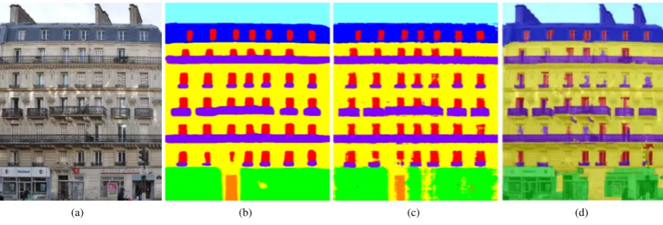
(a) (b) (c) (d)
Figure 1. Qualitative results of different methods. (a) shows the input image, (b) the output of our method and (c) the result of (Jampani et al., 2015) which is learned with boosted decision trees after three iterations of Auto-context (Tu, 2008). (d) depicts the
output of (Martinovi´c, 2015) which employs superpixel classification. The class labels are described in Fig. 2
Database (ECP) facade dataset (c.f. Section 5.1). In comparison, our approach takes less than 10 seconds per image. (Kozi´nski et al., 2014) first labels the facade using the facade segmentation method presented in (Cohen et al., 2014) and then the facade ob-jects are refined by grammar rules.
Current efficient methods for facade segmentation are based on the bottom-up paradigm. They usually consist of two parts. First, a pixelwise classification algorithm or a superpixel segmentation and classification algorithm with integrated object (window, door and car) detector is trained. In the second step, the labeled out-put image is optimized, noise reduced and the facade objects are delineated.
In (Cohen et al., 2014) a Dynamic Programming (DP) approach is used in an initial labeled image to find the optimal solution for facade segmentation. They employ hard architectural constraints between facade objects creating an iterative process that step by step defines facade objects. The algorithm is evaluated on the ECP dataset. Balconies and windows are defined in the first DP iteration, doors and shops in the second, and in the last roof and sky. They state that their algorithm performs in most cases very inaccurate for other images. This is because their DP approach encodes a very specific architectural facade style. On the other hand, their DP optimization algorithm is very fast and it takes on average 2.8 seconds per ECP facade image.
(Jampani et al., 2015) presents a classification method using Auto-context (Tu, 2008). They use three iterations of Auto-context in their algorithm and it produces quite accurate results. In their classifier, they employ in each iteration features from the output of the previous iteration. For each pixel they use class distributions, column and row statistics as well as entropy. The classifier consists of boosted decision trees learned by stacked generalization. In the classifier the output of the door and win-dow detectors is added as features. The Auto-context features can encode the density of the predicted class around the pixel as well as global characteristics. They lead to good results, but still the output of the classifier is noisy and contains non homogeneous segments. On average, the system takes around 5 seconds to la-bel an image of the ECP dataset. After three iterations of learning for the decision trees they employ a CRF to optimize and reduce the noise. The last step improves the results for about 1% and it reduces the noise but it takes another 24 seconds. The com-plete system takes around 30 seconds on average to label an ECP facade image.
In (Martinovi´c et al., 2012) a three layered approach for facade segmentation is described. In the first layer, a Recursive Neu-ral Network (RNN) is trained on an over-segmented facade. The output is a probability distribution for each pixel for all classes. In the second layer, window and door detectors are introduced. The output of the the detectors and the RNNs are incorporated in a Markov Random Field (MRF). The result of the MRF is still a noisy labeled image and does not follow the weak archi-tectural constraints. Thus, in the top layer they introduce weak and hard architectural constraints. The employed energy mini-mization method uses the architectural constraints as well as very particular architectural characteristics of the dataset such as that the second and the fifth floor have a running balcony.
The above authors have extended their work to the ATLAS ap-proach (Mathias et al., 2016). In the first layer the facade is seg-mented into superpixels, which are labeled by a classifier with one of the facade classes. Different segmentation methods and classifiers such as Multiclass Logistic Regression, CRF, Multi-layer Perceptron, Multiclass Support Vector Machine (SVM) and RNN have been evaluated. Their best first layer, using SVM, achieves an accuracy of 84.75% on the ECP dataset which is an improvement of around 2% compared to their previous work. The superpixel classification gives significantly higher accuracy for shops, roof and sky, but reduces the accuracy for doors. Thus, the SVM segmentation classification method is better in defining large objects and worse for small and less homogeneous objects. In the second layer, they improve their object detectors and in-troduce a car detector. The last layer is similar to (Martinovi´c et al., 2012). Overall, the final system has a pixelwise accuracy of 88.02%, which is an improvement of 3.85% compared to their previous work. The three layers take around 180 seconds to label an image of the ECP dataset.
3. STRUCTURED RANDOM FOREST
3.1 Decision Tree
The Decision Tree and Random Decision Forest are introduced and notations are given based on (Kontschieder et al., 2011a) and (Doll´ar and Zitnick, 2013).
A Decision Tree can be represented as ft(x) = y where x is an n-dimensional sample classified recursively by branch-ing down to the leaf node dependbranch-ing on the feature values of the sample x. The leaf node assigns the class y ∈ Y
to the data sample x. For our problem the data samples x
are image patches and their channel features, and the class la-bels are patches with pixels labeled with facade objectsY = ”window”,”door”,”wall”,”sky”, etc.
Each node of the tree decides if it branches left or right based on the split function defined as
h(x, θj)∈ {0,1} (1)
with parametersθj. If the functionh(x, θj)returns 0, then the node j is traversed down to the left, otherwise to the right. The recursive traversal terminates at the leaf nodes. The output of the tree for the samplexis the prediction stored in the leaf node where the traversal process terminated and a target labely∈ Y
or a distribution over the labels ofY.
The split function (Equation 1) can be complex. Yet, the most fre-quent choice is a simple function, where a single feature dimen-sion of samplexis compared to a threshold. Formallyθ= (k, τ)
wherekdefines the feature of the sample andτ the threshold. Then,h(x, θ) = [x(k)< τ], with[·]the indicator function. An-other often used split function ish(x, θ) = [x(k1)−x(k2)< τ] withθ= (k1, k2, τ).
3.2 Random Decision Forest
A Random Decision Forest is an ensemble ofTindependent trees
ft. For a samplexof the datasetDthe Random Decision Forest
F ofT trees gives the prediction as a combination of theft(x) witht∈1,2, ..Tusing an ensemble model such as majority vote or consensus. In the leaf nodes of each tree ofFarbitrary infor-mation about the model, which can help in the final decision of the prediction, is stored. The leaf node reached in each tree of
Fdepends only on the feature values ofx. The prediction of the Random Forest can be generated in an efficient way. The above characteristics allow to model complex output spaces, such as the structured outputs in (Kontschieder et al., 2011a)
3.3 Training of Decision Trees
The main goal of the training of trees is to find the best split functions (Equation 1) so that an as high as possible accuracy for the whole classification system is achieved. Formally, for a tree nodejand training setSj⊆X×Y we define parametersθj of the split function (Equation 1) to maximize the “quality” of the split. One possible measure of the split quality is the information gain
Ij=I(Sj, SjL, S R
j), (2)
whereSLj = (x, y)∈Sj|h(x, θj) = 0,SRj = Sj\SjL. The split parametersθjare chosen to maximizeIj. The training is recursively conducted for the left node with the dataSL
j and the right node withSjR. It ends when the predefined depth of the tree has been reached or the size ofSjfalls below a predefined
threshold. For a classification with multiple classes, the informa-tion gain is defined as: the probability distributionpyof the class elements in the subset
Sj.
3.4 Structured Random Forest
During the pixel labeling of the facade images, it is important to consider the local and global arrangement of the facade objects. There are architectural constraints and an object hierarchy that can be encoded in the classification algorithm.
In Standard Random Forests each pixel is assigned to a single class label independently of the neighboring pixels. This is the main cause that Standard Random Forests produce a noisy label-ing. The adaptation of structured learning (Nowozin and Lam-pert, 2011) to random forests allows to output a labeled patch and, thus, to strongly reduce the noise in image segmentation or labeling.
In comparison with Standard Random Forests, the Structured Random Forests output for each leaf node a patch with predefined dimensions and during the traversal of the tree the class labels of the neighboring pixels are also considered. The first means that each pixel is labeled from multiple patches, i.e., the label infor-mation is shared with the neighbors and the latter means that the split functions are constructed from two or more pixels.
Structured Random Forests struggle with the exponentially in-creased complexity of the output space. To overcome this draw-back, various methods have been proposed for the test and train-ing function selection, such as Principal Component Analysis (PCA) and probabilistic approaches (Kontschieder et al., 2014). In our approach the output of a leaf node is computed as a joint probability distribution of the labels assigned to the leaf node.
We use a training selection method similar to (Kontschieder et al., 2011a). It selects the best split function at each node based on the information gain with respect to two label joint distributions. The training works as follows: LetStbe the subset of the patches with dimension2d+ 1×2d+ 1and center(0,0)that is to be split at a tree node (t). We select the center pixel and a pixel in a random position(i, j)where|i|≤dand|j |≤dof the patch and compute the best split forSt for a featurex(k). The best split is chosen by computing the information gain ofSj. This continues recursively until the leaf node is reached (Kontschieder et al., 2011a, Kontschieder et al., 2014, Nowozin and Lampert, 2011).
4. OPTIMIZATION FOR STRUCTURED RANDOM FORESTS: THE LABEL PUZZLE GAME Since the Structured Random Forest outputs a patch with prede-fined dimensionsd×d, each pixel is covered byd2patches. Thus, each pixel is assignedd2values distributed over the classes. The pixel label is selected by majority vote.
select the best possible labeling for an image from the output patches of the trees of the forest. Let the ForestFhaveT trees and let the patchp(t)(i,j)be the predicted patch of the treetfor the pixel location with patch center(i, j). We defineagreement of the patchp(t)(i,j)as the number of correctly predicted pixels in the imagellabeled by the previous step.
φ(i,j)(p(t), l) = X
(r,c)∈p(t)
[p(t)(i,j)(r, c) =l(r, c)] (4)
For the next iteration, to label the patch with the center at the pixel
I(i, j)the tree with the highest agreement scoreφ(i,j)(p(t), l) is selected. In other words, from the forestF for each pixel the tree is chosen that has the most accurately labeled pixel in the predifined neighborhod (d×d). We perform this operation it-eratively. For this iterative model it has been proven that it con-verges to a local maximum with regard to the agreement function. For the complete proof and description of the method we refer to (Kontschieder et al., 2011b).
5. EXPERIMENTS 5.1 Datasets
ECPThis dataset contains 104 rectified facade images of Haus-mannian architectural buildings from Paris. The images are la-beled according to seven semantic classes (balcony, door, roof, shop, sky, wall and window– Fig. 2). The dataset has two ver-sions: The first version is presented by (Teboul et al., 2011) and the second by (Martinovi´c et al., 2012). In the first version all windows have the same width and are aligned on a grid. The sec-ond dataset is more accurate and provides the real position of the objects. In both datasets doors, windows, and shops are labeled as rectangles.
ParisArtDecoThis dataset is used and published by (Gadde et al., 2016). It contains 79 rectified facade images from Paris. As for the ECP dataset, the images are labeled according to seven semantic classes. We use this dataset only to train the door and window detectors.
GrazIt contains 50 rectified facade images of different architec-tural styles (Classicism, Biedermeier, Historicism, and Art Nou-veau) from Graz (Riemenschneider et al., 2012). The images are labeled according to four semantic classes (door, sky, wall and window– Fig.2).
(a) (b)
Figure 2. Label sets and colors for (a) ECP dataset (b) Graz dataset
5.2 Image Features
As image features we use RGB color, CIELab raw channels, His-togram of Oriented Gradients (HOG), location information, 17
TextonBoost filter responses and Local Binary Patterns. We ad-ditionally employ the per pixel score of the door and window detector of (Jampani et al., 2015), which is trained based on the integral channel feature detector (Dollar et al., 2009). The output are bounding boxes with corresponding scores and the scores are assigned to each pixel in the bounding box. In contrast to (Jam-pani et al., 2015) which trains the door and window detectors on the same dataset, we train them on the ParisArtDeco dataset and use it for the ECP and Graz dataset.
Since the facades are rectified, we add the per row variance and the median of the RGB channels as well as for each pixel the cor-responding deviation from the median value. We also employ the correlation coefficients between covariances of RGB raw channel intensities.
5.3 Evaluation
Our algorithm has been evaluated on the ECP and the Graz dataset. For both datasets we show the five-fold cross-validation results. The ECP dataset is divided in four sets with 20 images and one set with 24 images and the Graz dataset is divided in five sets of 10 images. To compare the results with (Jampani et al., 2015), we use the same configuration of sets. The Structured Random Forest is trained with a patch size of15×15pixels and a termination threshold of five samples for the leaf node.
Our empirical results (Fig. 4) are compared for the ECP dataset with the current four best bottom-up methods and for the Graz dataset (Fig. 3) with the results obtained by the method presented in (Jampani et al., 2015). We compare the two phases classifica-tion and optimizaclassifica-tion of our algorithm separately with the current state-of-the-art approaches.
Tables 1 and 3 give the evaluation results for the classifiers with-out optimization. We observe that our classification algorithm performs on par or even slightly better than the current best clas-sifiers. Particularly, our algorithm is significantly better for doors. Overall our classifier is better by about 1% than the other algo-rithms and produces results with less noise.
The optimization method relies just on the basic local arrange-ment of the facade objects. The global arrangearrange-ment is not consid-ered. Because of the local optimization, our algorithm delineates the objects efficiently (Fig. 5). Since we do not make any as-sumption about the global features and global arrangement of the facade objects, our algorithm is quantitatively (Tables 2 and 4) very slightly worse than the current state-of-the-art approaches.
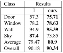
Class Results
Table 1. Labeling results of the classification stage on dataset Graz. Column (I) gives results from the first stage of Auto-context (Jampani et al., 2015). Ours: Structured Random
Forest only. Best results are given in bold.
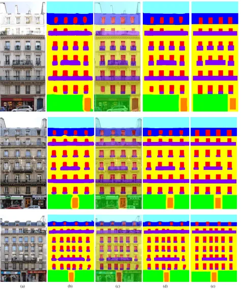
(a) (b) (c) (d) (e)
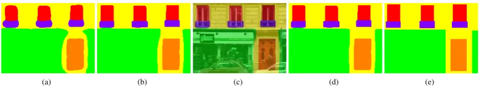
Figure 3. Qualitative results on the Graz dataset. The facade segments are homogeneous and nearly without noisy. Column (a) input images, (b) results from Structured Random Forest, (c) results after 10 iterations of the optimization algorithm mapped into the input
image, (d) results after 50 iterations and (e) ground truth. Colors see Fig. 2.
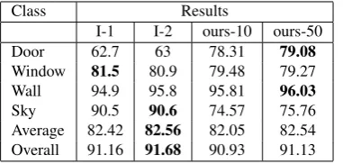
Class Results
I-1 I-2 ours-10 ours-50
Door 62.7 63 78.31 79.08
Window 81.5 80.9 79.48 79.27
Wall 94.9 95.8 95.81 96.03
Sky 90.5 90.6 74.57 75.76
Average 82.42 82.56 82.05 82.54 Overall 91.16 91.68 90.93 91.13 Table 2. Labeling results after optimization on dataset Graz.
Column (I-1) labeling optimized with three iterations of Auto-context (Jampani et al., 2015). (I-2) labeling optimized with Auto-context and CRF with an 8-connected neighborhood and pairwise Potts potentials. Ours-10 and Ours-50 after 10 and
50 iterations, respectively. Best results are given in bold.
a Structured Random Forest for facade labeling and have shown that the structured learning is efficient, because of its ability to learn the local structure of the facade objects. The experimental results on the ECP and Graz facade datasets demonstrate that it performs on par concerning certain aspects or even slightly better than state-of-the-art approaches. We presented an optimization algorithm which iteratively converges to the best possible label-ing. In the future we want to extend the optimization algorithm by adding constraints on the global structure of the facade and we want to speed it up. Additionally, we plan to develop a better object detector and features more specific for the problem.
7. ACKNOWLEDGEMENTS
This paper is supported by grant MA 1651/15 from Deutsche Forschungsgemeinschaft (DFG).
Class Results
I II-1 II-2 III-1 III-2 Ours
Door 76.2 43 60 41 58 83.77
Shop 87.6 79 86 91 97 94.61
Balcony 85.8 74 71 75 81 85.68
Window 77.0 62 69 64 76 79.20
Wall 91.9 91 93 91 90 91.32
Sky 97.3 91 91 94 94 95.98
Roof 86.5 70 73 82 87 90.76
Average 86.04 72.85 77.57 86.67 83.36 88.76 Overall 88.86 82.63 85.06 84.75 88.07 89.87 Table 3. Labeling results of the classification stages of various approaches on dataset ECP. Column (I) gives results for the first
stage of Auto-context (Jampani et al., 2015). (II-1) and (II-2) present results for the first and the second layer of the three-layered approach (Martinovi´c et al., 2012), respectively. (III-1) and (IV-1) show results for the first and the second layer
of ATLAS (Mathias et al., 2016). Best results are marked in bold.
REFERENCES
Cohen, A., Schwing, A. G. and Pollefeys, M., 2014. Efficient structured parsing of facades using dynamic programming. In: Computer Vision and Pattern Recognition, pp. 3206–3213.
Doll´ar, P. and Zitnick, C. L., 2013. Structured forests for fast edge detection. In: International Conference on Computer Vi-sion, pp. 1841–1848.
Dollar, P., Tu, Z., Perona, P. and Belongie, S., 2009. Integral channel features. In:British Machine Vision Conference, pp. 1– 11.
(a) (b) (c) (d) (e)
Figure 4. Qualitative results on the ECP dataset. The facade segments are homogeneous and nearly without noise. Column (a) input images, (b) results from Structured Random Forests, (c) results after 10 iteration of the optimization algorithm mapped in the input
Class Results
I-1 I-2 II III IV Ours-10 Ours-50
Door 80.4 81.3 67 71 79 82.16 79.47
Shop 91.6 93.2 93 95 94 94.85 95.17
Balcony 89.4 89.3 70 87 91 88.38 86.43
Window 81.8 82.3 75 78 85 80.54 80.41
Wall 92.4 92.9 88 89 90 91.47 91.52
Sky 98.0 98.2 97 96 97 96.15 96.18
Roof 88.1 89.2 74 79 93 90.98 91.02
Average 88.79 89.49 80.71 85.22 89.4 88.93 88.60 Overall 90.81 91.42 84.17 88.02 90.82 90.21 90.24
Table 4. Labeling results after optimization for various approaches on dataset ECP. Column (I-1) gives results for Auto-context (Jampani et al., 2015) after three iterations and (I-2) for Auto-context with CRF with an 8-connected neighborhood and pairwise Potts
potentials. (II) presents the third layer of the three layered approach (Martinovi´c et al., 2012) for facade parsing and (III) ATLAS (Mathias et al., 2016), respectively. (IV) gives results for the DP optimization approach (Cohen et al., 2014). The end results of our
method after 10 and 50 iterations are given by Ours-10 and Ours-50, respectively. Best results are marked in bold.
(a) (b) (c) (d) (e)
Figure 5. Iterative delineation. Image (a) results from the Structured Random Forest. (b) gives results after 10 iterations, (c) results after 10 iterations mapped into the input image, (d) results after 50 iterations and (e) ground truth. One can observe that the object
delineation is very accurate even after only the 10th iterations. Colors see Fig. 2.
Jampani, V., Gadde, R. and Gehler, P. V., 2015. Efficient facade segmentation using auto-context. In:IEEE Winter Conference on Applications of Computer Vision, pp. 1038–1045.
Kontschieder, P., Bulo, S. R., Bischof, H. and Pelillo, M., 2011a. Structured class-labels in random forests for semantic image labelling. In: International Conference on Computer Vision, pp. 2190–2197.
Kontschieder, P., Bul`o, S. R., Donoser, M., Pelillo, M. and Bischof, H., 2011b. Semantic image labelling as a label puzzle game. In:British Machine Vision Conference, pp. 1–12.
Kontschieder, P., Bulo, S. R., Pelillo, M. and Bischof, H., 2014. Structured labels in random forests for semantic labelling and ob-ject detection. IEEE Transactions on Pattern Analysis and Ma-chine Intelligence36(10), pp. 2104–2116.
Kozi´nski, M., Obozinski, G. and Marlet, R., 2014. Beyond proce-dural facade parsing: Bidirectional alignment via linear program-ming. In:Asian Conference on Computer Vision, pp. 79–94.
Martinovi´c, A., 2015. Invers procedural modeling. Technical re-port, Arenberg Doctoral School Faculty of Engineering Science, KU Luven.
Martinovi´c, A., Mathias, M., Weissenberg, J. and Van Gool, L., 2012. A three-layered approach to facade parsing. In:European Conference on Computer Vision, pp. 416–429.
Mathias, M., Martinovi´c, A. and Van Gool, L., 2016. ATLAS: A Three-Layered Approach to Facade Parsing.International Jour-nal of Computer Vision118(1), pp. 22–48.
Mayer, H. and Reznik, S., 2006. MCMC Linked with Implicit Shape Models and Plane Sweeping for 3D Building Facade Inter-pretation in Image Sequences”. In:International Archives of the Photogrammetry, Remote Sensing and Spatial Information Sci-ences, Vol. (36) 3, pp. 130–135.
Nowozin, S. and Lampert, C. H., 2011. Structured learning and prediction in computer vision. Foundations and TrendsR in
Computer Graphics and Vision6(3–4), pp. 185–365.
Reznik, S. and Mayer, H., 2008. Implicit Shape Models, Self Di-agnosis, and Model Selection for 3D Facade Interpretation. Pho-togrammetrie – Fernerkundung – Geoinformation3/08, pp. 187– 196.
Riemenschneider, H., Krispel, U., Thaller, W., Donoser, M., Havemann, S., Fellner, D. and Bischof, H., 2012. Irregular lat-tices for complex shape grammar facade parsing. In: Computer Vision and Pattern Recognition, pp. 1640–1647.
Teboul, O., Kokkinos, I., Simon, L., Koutsourakis, P. and Para-gios, N., 2011. Shape grammar parsing via reinforcement learn-ing. In: Computer Vision and Pattern Recognition, pp. 2273– 2280.
Teboul, O., Simon, L., Koutsourakis, P. and Paragios, N., 2010. Segmentation of building facades using procedural shape priors. In:Computer Vision and Pattern Recognition, pp. 3105–3112.