EXTERIOR ORIENTATION OF HYPERSPECTRAL FRAME IMAGES COLLECTED
WITH UAV FOR FOREST APPLICATIONS
A. Berveglieri a and A. M. G. Tommaselli b
a, b
Univ Estadual Paulista – UNESP, Faculty of Science and Technology, Presidente Prudente, Brazil, a
Graduate Program in Cartographic Sciences, b Department of Cartography a
[email protected], b [email protected]
KEY WORDS: Forest, Hyperspectral Image, Orientation, Sparse Control, UAV
ABSTRACT:
This paper describes a preliminary study on the image orientation acquired by a hyperspectral frame camera for applications in small tropical forest areas with dense vegetation. Since access to the interior of forests is complicated and Ground Control Points (GCPs) are not available, this study conducts an assessment of the altimetry accuracy provided by control targets installed on one border of an image block, simulating it outside a forest. A lightweight Unmanned Aerial Vehicle (UAV) was equipped with a hyperspectral camera and a dual-frequency GNSS receiver to collect images at two flying strips covering a vegetation area. The assessment experiments were based on Bundle Block Adjustment (BBA) with images of two spectral bands (from two sensors) using several weighted constraints in the camera position. Trials with GCPs (presignalized targets) positioned only on one side of the image block were compared with trials using GCPs in the corners. Analyses were performed on altimetry discrepancies obtained from altimetry checkpoints. The results showed a discrepancy in Z coordinate of approximately 40 cm using the proposed technique, which is sufficient for applications in forests.
1. INTRODUCTION
The monitoring of recovered and native forests is a widely recognized global need which requires updated geospatial information. Aerial and orbital imagery can be used for large areas but the spatial and temporal resolutions are limited and these techniques are not cost-effective for small areas.
In remaining forests, for example, the use of images collected by Unmanned Aerial Vehicles (UAVs) is feasible due to the lower costs and the possibility of images acquisition with suitable spatial and temporal frequency. In recent years, UAVs have been increasingly adopted as platforms for applications of photogrammetry and remote sensing, as discussed by Colomina and Molina (2014). Remondino et al. (2011) reported some UAV systems for photogrammetric applications as well as Eisenbeiss (2011) who described the potential of UAVs for mapping tasks.
New types of hyperspectral sensors have been introduced to UAV applications, such as the Rikola camera with a Fabri-Perot interferometer (FPI), which acquires sequence 2D images in frame format. A review presented by Aasen et al. (2015) reported important studies and the potentiality of hyperspectral sensors to derive information, e.g., about vegetation, plant diseases, environmental conditions, and forest. Honkavaara et al. (2013) performed experiments using UAV with a FPI-based hyperspectral camera to collect hyperspectral and structural information and to estimate plant height and biomass. The trials demonstrated great potential for precision agriculture and indicated feasibility for other research topics.
In spite of the instability of UAV platforms, accurate data can be provided depending on the requirements, as commented by Eisenbeiss (2011), which enables the use of UAVs in
inaccessible areas, for example, forests. However, ground control is required to indirectly orient the images, although this task could be complicated in areas with dense vegetation such as tropical forests.
Considering these needs this study performed a preliminary assessment on the image orientation in vegetation area using images acquired with a hyperspectral frame camera (Rikola) on board a lightweight UAV with a dual-frequency GNSS receiver for image georeferencing. The main purpose is to assess the results of hyperspectral image orientation using sparse ground control only at the beginning of flying strips, i.e., simulating a configuration outside forest areas.
The experiments were conducted using presignalized targets arranged along the flight trajectory over a vegetation area. The altimetry accuracy obtained with Bundle Block Adjustment (BBA) was analysed based on the discrepancies at altimetry checkpoints, which demonstrated the feasibility of the proposed technique.
2. HYPERSPECTRAL FRAME CAMERA
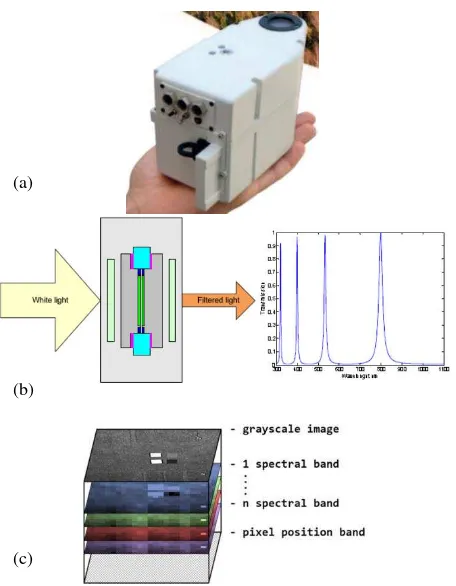
The Rikola company has made a 2D hyperspectral frame camera based on FPI with a RGB-NIR sensor, as shown in Figure 1(a). This FPI into the lens system is used to collimate the light, and then the spectral bands are a function of the interferometer air gap. Changes in the air gap enable to acquire a set of wavelengths for each image (Figure 1(b)). The range of air gap in FPI can provide wavelengths from 500 nm to 900 nm using two CMOS image sensors.
After acquiring images, the data is converted from analog to digital in 16-bit. Time information, collected by GPS receiver, is recorded for each image trigger and can be synchronized by a
microcontroller to work in time interval based self-triggering mode. Both GPS position and irradiance data are recorded.
Figure 1: (a) Hyperspectral frame camera. (b) Fabry-Perot principle. (c) Image data cube. Source: adapted from (b) Rikola
Ltd. and (c) Aasen et al. (2015).
The hyperspectral camera acquires the images as binary data cube with a number of bands using a predefined sequence of air gap values to reconstruct the spectrum of each pixel in the image, as described by Honkavaara et al. (2013) and depicted in Figure 1(c). Each data cube (or image) has information on the wavelengths of bands, radiometry, and pixel position.
According to Mäkeläinen et al. (2013), hyperspectral frame sensors are suitable for lightweight UAV imaging, since the sensor has approximately 600 g. In addition, the images in frame format allow conventional aerial triangulation for exterior orientation determination, which is essential for photogrammetric application that requires accurate results.
In general, photogrammetric projects with that type of sensor are planned with UAVs at heights of 100-200 m, resulting in a GSD of 5-15 cm, which is sufficient for UAV application as agriculture and forest canopy monitoring.
3. METHODOLOGY
The methodology is based on the assessment of minimum configuration of ground control for small forest areas, refining the camera Perspective Centre (PC) positions collected during the flying survey . The following sections describe the required steps.
3.1 Camera calibration
The first step is the camera calibration, since accurate data are needed. Typically focal length (f), principal point (x0, y0) and
lens distortion coefficients (K1, K2, K3, P1, P2) are the
parameters to be determined, which define the Interior Orientation Parameters (IOPs). The mathematical model is based on the collinearity equations (Kraus, 2007) with addition of parameters of the Conrady-Brown model (Fryer and Brown, 1986).
The estimation of the IOPs can be done by a self-calibrating bundle adjustment considering constraints imposed to the ground coordinates, as proposed by Kenefick et al (1972).
3.2 Positioning of control targets and GNSS surveying
Ground control points are used to indirectly estimate EOPs or to refine the observed values when using GNSS to determine the coordinates of the exposure stations. Usually such control is planned to be distributed in the block borders (Kraus, 2007).
In tropical forests, GCPs are not available or suitable areas to set them up can be inaccessible due to dense vegetation, which complicates the acquisition of ground coordinates and the visibility from aerial images. Thus, a few presignalized targets or natural points have to be used as ground control outside the forest or in clearings. Depending of the vegetation features natural points are scares on unsuitable to be used. Considering that UAV operation is always on site it is straightforward to install signalised target around the take-off and landing area. These targets are installed before the flying survey and will be used to improve the PC coordinates determined with GNSS. A GNSS base station is also defined close to the GCPs to improve the GNSS post-processed solution since real time GNSS network are not dense in Brazil.
3.3 Image data acquisition
The aerial survey is planned to acquire hyperspectral images over a forest area. The camera PC positions are determined by a GNSS receiver during the flight using a reference band of the image cube, which is defined by the camera manufacturer. Since the attitude angles are not directly determined, they are later estimated in the image orientation by BBA using initial values from the flight plan.
3.4 Image orientation
The image cube is formed by a set of spectral bands that can be oriented separately. For image orientation, the image frames are connected with tie points to enable the BBA from a minimum of GCPs and weighted constraints in the camera PC positions. The dual-frequency GNSS receiver installed on board UAV allows the acquisition of accurate PC positions during the aerial survey. The attitude angles were considered as unknowns. The control targets are used as GCPs considering the accuracy resulting from GNSS surveying.
4. EXPERIMENTS AND RESULTS
This section describes the methodology to perform an aerial survey to collect hyperspectral frame images over a vegetation area. The experiments were performed to assess the resulting accuracy of the image orientation using GCPs only in one side of the image block, which is likely to occur in UAV flights over forest areas. The results were compared with those achieved when using GCPs in the border corners.
(a)
(b)
(c)
4.1 Performing terrestrial camera self-calibration
The camera self-calibration procedure was performed in a 3D terrestrial calibration field composed of coded targets with Aruco format (Garrido-Jurado et al., 2014). These targets were automatically located in the images using a software adapted by Silva et al. (2014) that identifies each target image coordinate with its respective ground coordinate.
A total of twelve images was captured for camera calibration using the hyperspectral camera specified in Table 1. Previously the camera was configured to acquire data cubes with twenty five spectral bands, more details in Tommaselli et al. (2015).
Camera model Rikola FPI2014
Nominal focal length 9 mm
Pixel size 5.5 μm
Image dimension 1023 × 648 Table 1. Technical details.
The images were collected from several camera stations in the calibration field using different positions and rotations to avoid correlation between IOPs and EOPs. Figure 2 exemplifies two images with Aruco target identified, which were used in the camera calibration procedure.
Figure 2. Hyperspectral images with Aruco targets identified. Both images were used in the camera calibration procedure.
Two spectral bands (one of each sensor, 605.64 nm and 689.56 nm) were selected for camera self-calibration. The procedure was performed with seven constraints in the object space. The coordinates of two ground points were fixed (X1, Y1, Z1, X2, Y2, Z2) and a Z coordinate of a third point (Z3) orthogonal to these two previous points. IOPs and EOPs were considered as unknowns in the BBA procedure, being calculated by the calibration multi-camera (CMC) software (developed in-house by Ruy et al. (2009)). The estimated values of the IOPs and the a posteriori sigma are presented in Table 2.
Parameter
Sensor 1 (689.56 nm) Sensor 2 (605.64 nm)
Estimated value
Standard deviation
Estimated value
Standard deviation
f (mm) 8.6905 0.0118 8.6488 0. 0321
x0(mm) 0.4165 0.0050 0.3665 0.0138
y0(mm) 0.3997 0.0039 0.4365 0.0107
K1(mm-2) -4.74×10⁻³ 1.06×10⁻⁴ -4.13×10⁻³ 3.04×10⁻⁴
K2(mm-4) -1.78×10⁻⁶ 2.21×10⁻⁵ -6.34×10⁻⁵ 6.54×10⁻⁵
K3 (mm-6) -6.71×10⁻⁷ 1.43×10⁻⁶ 4.75×10⁻⁶ 4.37×10⁻⁶
P1 (mm-1) -2.86×10⁻⁵ 8.85×10⁻⁶ -1.73×10⁻⁴ 2.48×10⁻⁵
P2 (mm-1) -1.15×10⁻⁴ 1.17×10⁻⁵ -3.06×10⁻⁴ 3.19×10⁻⁵
a posteriori sigma (a priori = 1)
0.06 0.43
Table 2. IOPs determined by self-calibration.
4.2 Aerial survey
Before carrying out the aerial survey, five presignalized control targets, as shown in Figure 3(a), were geometrically positioned along the border of the test area. Figure 4(b) displays the block geometry and Figure 3(b) shows an example of the control target appearing in the image.
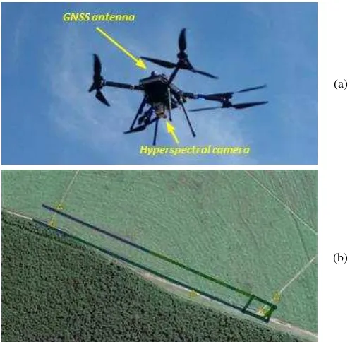
Sensormap Company performed the aerial survey using a lightweight UAV (octopter) platform equipped with the Rikola hyperspectral camera and a dual-frequency GNSS receiver, as shown in Figure 4(a).
(a) (b)
Figure 3. (a) GNSS surveying using a presignalized target. (b) Control target appearing in the aerial hyperspectral image.
The hyperspectral camera was configured to acquire spectral image cubes at a flying height of 160 m with flying speed of 4 m/s. Two flying strips were collected covering a range of 800 m over a vegetation area (composed of forest and sugarcane, as shown in Figure 4(b)), which resulted in images with a GSD of 11 cm. The flight planning was performed with longitudinal and lateral overlap of 80% and 30%, respectively.
(a)
(b)
Figure 4. (a) UAV equipped with a hyperspectral camera and GNSS receiver. (b) Distribution of five GCPs (triangles) and trajectory followed by the UAV to acquire hyperspectral
images.
4.3 Bundle adjustment
Considering the same two spectral bands selected for the camera calibration, two blocks were formed with the corresponding images and BBA was performed for each block using ERDAS Imagine – LPS software (v. 2015) with the following configuration:
• Initial positions of the camera PC were based on the data collected with GNSS receiver and processed by differential positioning technique with the base station on site (weighted constraints varying from 10 cm to 50 cm were used) and attitude angles were considered as unknowns;
• Calibrated IOPs were considered as absolute constraints; • Image coordinates (automatically extracted) with standard
deviation of 1/2 pixels;
• GCPs were surveyed in the midpoint between the two circular target centroids, and used with a standard deviation of 5 cm, based on the GNSS positioning accuracy.
Each GCP was located in one image and then transferred to homologue positions in the adjacent images using least squares matching via LPS software. Tie points were automatically generated using 25 points per model (default distribution).
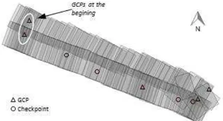
Figure 5. Image block geometry with 93 images, five GCPs, and four altimetry checkpoints.
One of the advantages in using presignalised targets is the automatic centre location that enables to achieve a better precision. In this project, the targets centroids were automatically located in the images and, from them, the midpoint corresponding to the GCP. This strategy was used to minimize measurement errors caused by image blurring and saturation.
It is important to note that all spectral bands are not simultaneously recorded at the same exposure time. The time interval from band to band is approximately 22 ms and image bands are grabbed sequentially with the platform displacement. Thus, the camera PC positions have to be interpolated for the selected spectral bands under study using the GPS time of a first acquired default band. The time interval for each band is determined by a sequence delay calculator provided by Rikola Company. The GPS time of the default band is grabbed by a navigation single frequency GPS integrated to the Rikola camera.
4.4 Results
Considering the band selected in the sensor 1 (689.56 nm), Figure 6 presents a graph generated with the root mean square error (RMSE) of GCPs resulting from the BBA for different weighted constraints in the camera PC position. As shown in Figure 5, five GCPs (in the corners) were used in the experiment to be compared when using two GCPs only at the beginning of the flying strips (see Figure 5).
Figure 6. Sensor 1 – RMSE for GCPs resulting from the BBA considering GCPs in the corners and only on one side of the
image block.
The results indicated larger RMSEs when GCPs were only used in one side of the image block, presenting values of 0.460-0.053 m in X and 0.035-0.046 m in Y. For the case with GCPs in the corners, the RMSEs were smaller varying 0.034-0.041 m in X e 0.027-0.038 m in Y. The Z coordinate presented approximate RMSEs < 0.01 m, which is better than XY and can be explained by the blurring affecting the measurements in the X direction. Another problem not yet assessed is the event logging error.
Figure 7 shows the RMSEs at GCPs with respect to the BBA for the sensor 2 (spectral band of 605.64 nm). When GCPs were only used on one side, the RMSEs were larger, 0.045-0.049 m in X and 0.069-0.076 m in Y. The larger errors presented in Y can be an effect caused by image blurring, which is more likely to occur in the sensor 2 (visible spectrum). With GPCs in the corners, the RMSEs were 0.031-0.38 m in X and 0.041-0.045 m in Y. In relation to Z coordinate, the errors were quite similar, being below 0.01 m.
Figure 7. Sensor 2 – RMSE of GCPs resulting from the BBA considering GCPs in the corners and only on one side of the
image block.
Comparing the results with GCPs in the corners and GCPs only on one side, the largest differences (in both graphs) were verified in the planimetry and the better results were obtained with GCPs in the corners, as expected. However, even using GCPs in one side, the RMSEs were smaller than 8 cm (< 1 GSD = 11 cm). Comparing the RMSEs in the five ranges of weighted constraints for the camera position, the RMSEs presented a slight decreasing value in planimetry following the ranges. This can be explained by errors in XY components of the PC coordinates which were probably caused by the time stamp provided by Rikola, blurring or by changes in the IOPs.
In the image space, the BBA produced sub-pixel residuals ranging between 0.25 and 0.40 pixels in all cases. In relation to the a posteriori sigma, Table 3 presents the sigma values for the several weighted constraints used in the camera position in both configurations of GCPs. Although the sigma values with GCP on one side are smaller in comparison with GCP in the corner, the differences are negligible.
Weighted constraint in the camera PC position
A posteriori sigma 10
cm 20 cm
30 cm
40 cm
50 cm
Sensor 1 GCP in the corner 0.57 0.57 0.55 0.54 0.53
GCP in one side 0.56 0.55 0.54 0.53 0.52
Sensor 2 GCP in the corner 0.54 0.53 0.53 0.52 0.51
GCP in one side 0.53 0.52 0.52 0.51 0.50
Table 3. A posteriori sigma in the BBA (a priori sigma = 0.50).
Another analysis can be made to assess the accuracy in altimetry. Four independent altimetry checkpoints were used to calculate the RMSE in Z coordinate. The planimetry errors were not assessed because these checkpoints were reused from a previous field survey and were not signalized for this hyperspectral flight. However, for forest application, the most critical errors are in heights, which can affect the modelling of forest canopy structure.
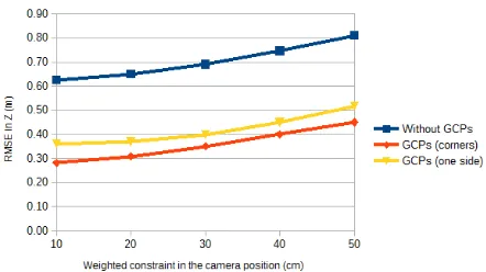
The graph in Figure 8 shows the RMSEs produced by the BBA using five weighted constraints in the camera position of the sensor 1. Three GCP configurations were used: without GCPs (only camera positions from GPS), integrated image orientation with GCPs in the corners, and integrated image orientation with GCPs at the beginning of the two flying strips.
Figure 8. Sensor 1 – RMSE in Z coordinate calculated with four altimetry checkpoints in the BBA.
The RMSEs obtained without GCPs only using the camera PC positions generated altimetry discrepancies from 0.64 m up to 0.85 m depending on the weighted constraint. The use of GCPs showed to be important to improve the accuracy in Z. Using GCPs only on side yielded RMSEs from 0.34 m up to 0.69 m, while GCPs in the corner resulted in RMSEs from 0.29 m up to 0.43 m. The two curves (red and yellow) indicated smaller differences for the weighted restrictions below 30 cm, equivalent to differences around 1 GSD. Above the constraint of 30 cm, the RMSEs were larger and showed an increasing tendency.
Figure 9 presents the RMSEs at altimetry checkpoints for the sensor 2 which is similar to sensor 1. The BBA without GCPs generated RMSEs from 0.63 m to 0.81 m. Such RMSEs were improved using the GCPs in the corners, which presented altimetry discrepancies of 0.28-0.45 m. The GCPs only on one side resulted in RMSEs from 0.36 m to 0.52 m. In the comparison between the yellow and red curves, the differences were smaller than 1 GSD, showing less sharp curves for weighted constraints below 30 cm. Above 30 cm, a sharp increasing tendency of the RMSEs was observed.
Figure 9. Sensor 2 – RMSE in Z coordinate calculated with four altimetry checkpoints in the BBA.
Based on the graphical analysis from Figures 8 and 9, the weighted restrictions below 30 cm presented the most suitable value for the configuration of the image block processing with sparse control, which resulted in altimetry discrepancies smaller than 40 cm.
The assessment based on RMSEs show that weighted constraints as it was expected are mandatory in the proposed technique and can produce acceptable results with few points in one strip side. Thus, a sparse ground control for forest applications can be used, when control targets can only be positioned outside the mapping area.
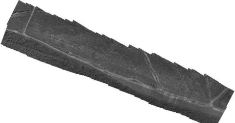
Figure 10 displays a mosaic generated with the images of a spectral band under study (605.64 nm). From the image orientation of this band, other spectral bands from the same sensor can be co-registered with relation to this one. Some radiometric effects can be observed in the mosaic, which was caused by illumination variations (cloud shadows) during the image acquisition.
Figure 10. Mosaic generated with the spectral band (605.64 nm, sensor 2) in study. Some radiometric effects can be realized due
to the illuminarion variation during the flying survey.
5. CONCLUSIONS
This study presented a preliminary experiment on the hyperspectral frame image orientation for forest applications using UAV. The main objective was to assess the altimetry accuracy provided by using only sparse control outside the forest.
The experiments were based on the BBA of two hyperspectral bands (two sensors) using two flying strips collected with UAV which is the expected configuration for the future flights. Control targets were installed in a vegetation area to assess the feasibility of using only ground controls at the beginning of flying strips, simulating them outside the forest. The trials considered GCPs positioned in the image block corners and GCPs only on one border.
The analysis of results was based on altimetry discrepancies obtained from four altimetry checkpoints and discrepancies in the GCPs. The RMSEs showed that ground control is needed to improve accuracy for the case studied, which was verified in the comparison of RMSEs without using GCPs and RMSEs with GCPs in the BBA. When the BBA using GCPs in the corners was compared with GCPs in one border, the RMSE differences (Figures 8 and 9) presented approximately 1 GSD between the curves (yellow and red) for weighted constraints below 30 cm in the camera position.
In general, the preliminary results of both spectral bands presented a discrepancy of approximately 40 cm in Z coordinate, which is sufficient for photogrammetric applications in forests, such as DSM generation and vegetation mapping. For future studies, the planimetry accuracy in checkpoints should be assessed, as well as the optimum number of GCPs at the beginning of flying strips and other image block arrangements. The stability of the IOPs in the image orientation should also be investigated as well as suitable configurations of flight strips and GCP to enable on-the-job calibration.
ACKNOWLEDGEMENTS
The authors would like to thank the São Paulo Research Foundation (FAPESP) – grants 2014/05533-7 and 2013/50426-4 and Sensormap Company for providing aerial images.
REFERENCES
Aasen, H., Burkart, A., Bolten, A. and Bareth, G., 2015. Generating 3D hyperspectral information with lightweight UAV
snapshot cameras for vegetation monitoring: from camera calibration to quality assurance. ISPRS Journal of Photogrammetry and. Remote Sensing. 108, pp. 245 – 259.
Colomina, I. and Molina, P., 2014. Unmanned aerial systems for photogrammetry and remote sensing: a review. ISPRS Journal of Photogrammetry and. Remote Sensing. 92(6), pp. 79 – 97.
Eisenbeiss, H., 2011. The potential of unmanned aerial vehicles for mapping. In: Photogrammetrische Woche 2011. Fritsch, D., pp. 135–145.
Fryer, J.G. and Brown, D.C., 1986. Lens distortion for close-range photogrammetry. Photogrammetric Engineering & Remote Sensing. 52(1), pp. 51–58.
Garrido-Jurado, S., Muñoz-Salinas, R., Madrid-Cuevas, F.J. and Marín-Jiménez, M.J., 2014. Automatic generation and detection of highly reliable fiducial markers under occlusion. Pattern Recognition. 47(6), pp. 2280 – 2292.
Honkavaara, E., Saari, H., Kaivosoja, J., Pölönen, I., Hakala, T., Litkey, P., Mäkynen, J. and Pesonen, L., 2013. Processing and assessment of spectrometric, stereoscopic imagery collected using a lightweight UAV spectral camera for precision agriculture. Remote Sensing. 5(10), pp. 5006–5039.
Kenefick, J. F., Gyer, M. S., Harp, B. F., 1972. Analytical self-calibration. Photogrammetric Engineering, 38, 1117–1126.
Kraus, K., 2007. Photogrammetry: geometry from images and laser scans, 2nd ed. de Gruyter, Berlin. 459 p.
Mäkeläinen, A., Saari, H., Hippi, I., Sarkeala, J. and Soukkamäki, J., 2013. 2D hyperspectral frame imager camera data in photogrammetric mosaicking. In: The International Archives of the Photogrammetry, Remote Sensing and Spatial Information Sciences. Rostoch, Germany. . XL-1/W2, pp. 263– 267.
Remondino, F., Barazzetti, L., Nex, F., Scaioni, M. and Sarazzi, D., 2011. UAV photogrammetry for mapping and 3D modeling - current status and future perspectives, In: The International Archives of the Photogrammetry, Remote Sensing and Spatial Information Sciences. Zurich, Switzerland. Vol. XXXVIII-1/C22, 7 pages.
Ruy, R., Tommaselli, A.M.G., Galo, Maurício, M., Hasegawa, J.K. and Reis, T.T., 2009. Evaluation of bundle block adjustment with additional parameters using images acquired by SAAPI system In: Proceedings of 6th International Symposium on Mobile Mapping Technology. Presidente Prudente, Brazil.
Tommaselli, A. M. G., Berveglieri, A., Oliveira, R. A., Nagai, L. Y., Honkavaara, E., 2015. Orientation and calibration requirements for hyperpectral imaging using UAVs: a case study. In: Proceeding of the Calibration and Orientation Workshop – EuroCOW 2015. Lausanne, Switzerland, February 10-12, 8 pages.
Silva, S.L.A., Tommaselli, A.M.G. and Artero, A.O., 2014. Utilização de alvos codificados na automação do processo de calibração de câmaras. Boletim de Ciências Geodésicas. 20(3), pp. 636–656.